Week 2 Air standard Cycle
the otto cycle explains the working of the piston inside the cylinder with respect to the given inputs
it has four stages 1 to 4.
the working is defined by the changes happening between them.
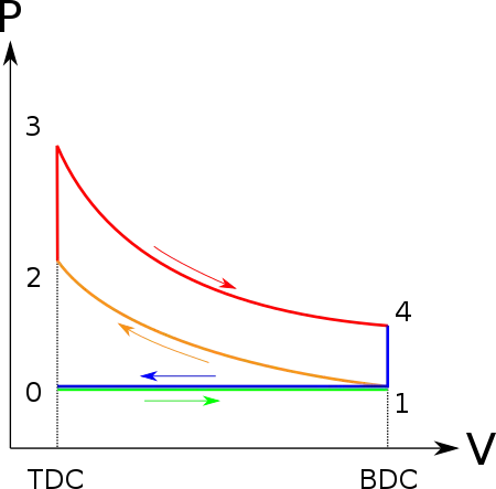
Process 0–1 a mass of air is drawn into piston/cylinder arrangement at constant pressure.
Process 1–2 is an adiabatic (isentropic) compression of the charge as the piston moves from bottom dead center (BDC) to top dead center (TDC).
Process 2–3 is a constant-volume heat transfer to the working gas from an external source while the piston is at top dead center. This process is intended to represent the ignition of the fuel-air mixture and the subsequent rapid burning.
Process 3–4 is an adiabatic (isentropic) expansion (power stroke).
Process 4–1 completes the cycle by a constant-volume process in which heat is rejected from the air while the piston is at bottom dead center.
Process 1–0 the mass of air is released to the atmosphere in a constant pressure process.
this process helps in easy understanding of the working of piston inside the engine.
MAIN PYTHON CODE:
#importing the main modeules like math and matplotlib for the correct functioning of te commands
import math
import matplotlib.pyplot as plt

#engine kinematics
def engine_kinematics(bore,stroke,con_rod,cr,start_crank,end_crank):
	#crank pin value
	a = stroke/2
	#value of R
	R = con_rod/a

	#volume of the stroke or the volume traced by the piston
	v_s = (math.pi/4)*pow(bore,2)*stroke
	#clearence volume ot the volume above the top dead center
	v_c = v_s/(cr-1)

	#starting crank angle and ending crank angle
	s_c = math.radians(start_crank)
	e_c = math.radians(end_crank)

	#number of divisions or points required to trace a smooth curve
	num_values = 100

	dtheta = (e_c - s_c)/(num_values-1)

	V = []

	for i in range(0,num_values):
		theta = s_c + i*dtheta
	    #the formula is breaken to easy understanding into 3 terms
		term1 = 0.5*(cr-1)
		term2 = R+1-math.cos(theta)
		term3 = (pow(R,2)- pow(math.sin(theta),2))
		term3 = pow(term3,0.5)
		V.append((1+term1*(term2 - term3))*v_c)

	return V


#inputs for the code is stated
#the pressure and the temperature at the point 1 is
p1 = 101325
t1 = 500
#gamma value
gamma = 1.4
#temperature for the point three is stated
t3 = 2300

#engine specs

#the top surface or the bore
bore = 0.1
#stroke that is the side face of the piston
stroke = 0.1
#connecting rod or con rod
con_rod = 0.15
#compression ratio
cr = 12


#volume of the stroke or the volume traced by the piston
v_s = (math.pi/4)*pow(bore,2)*stroke
#clearence volume ot the volume above the top dead center
v_c = v_s/(cr-1)


#volume at the point 1
v1 = v_s+v_c

#at state point 2
v2 = v_c
#the value of p2 is obtained from p2*v2^gamma = p1*v1^gamma
p2 = p1*pow(v1,gamma)/pow(v2,gamma)

#the value of t2 is obtained from p1*v1/t1 = p2*v2/t2
rhs = p1*v1/t1
t2 = p2*v2/rhs

#the compression of the pressure and volume after the 1nd state point is stated
v_compression = engine_kinematics(bore,stroke,con_rod,cr,180,0)

constant = p1*pow(v1,gamma)

#the  compression points are stated here with the help of the for loop below
p_compression = []

for v in v_compression:
	p_compression.append(constant/pow(v,gamma))

#at state point 3
#volume is similar to 2 so
v3 = v2
#from p2*v2/t2 = p3*v3/t3, rhs = p2*v2/t2. so
rhs = p2*v2/t2
p3 = rhs*t3/v3

#the expansion of the pressure and volume after point 3 is stated
v_expansion = engine_kinematics(bore,stroke,con_rod,cr,0,180)

constant = p3*pow(v3,gamma)

#the  expansion points are stated here with the help of the for loop below
p_expansion = []

for v in v_expansion:
	p_expansion.append(constant/pow(v,gamma))

#at state point 4
#the volume is similar to the point 1, so
v4 = v1
#from p3*v3^gamma = p4*v4^gamma
p4 = p3*pow(v3,gamma)/pow(v4,gamma)
#from p4v4/t4 = p3v3/t3,rhs = p3v3/t3
t4 = p4*v4/rhs

#plotting of the pv diagram is done
plt.plot([v2,v3],[p2,p3],'g')
plt.plot(v_compression,p_compression,'r')

plt.plot(v_expansion,p_expansion,'b')
plt.plot([v4,v1],[p4,p1],'y')
plt.title('PV DIAGRAM OF OTTO CYCLE')
plt.xlabel('Volume (m^3/s)')
plt.ylabel('Pressure (Pa)')
plt.show()


#thermal efficiency of the otto cycle
n = 1 - (pow(cr,(1-gamma)))
print(n)
EXPLANATION FOR THE CODE:
the important modules for the function to understand the commands given as an input is taken in with the help of the import command.
#importing the main modeules like math and matplotlib for the correct functioning of te commands.
math helps in basic calculations
import math
matplotlib helps in plotting of the results.
import matplotlib.pyplot as plt
the engine kinematics function contains thhe important aspects for the motion of the piston inside the cylinder. it contains the name of the function, value of the bore, stroke,conn_rod, cr, start_crank, end_crank.
#engine kinematics
def engine_kinematics(bore,stroke,con_rod,cr,start_crank,end_crank):
R and a is helpful in the tracing of compression and expansion of the piston
a is the pin that connect the connecting rod and crank shaft.
#crank pin value
a = stroke/2
R is the ratio of the con rod value and crank pin value.
#value of R
R = con_rod/a
it is the region in which the piston moves inside the cylinder.
#volume of the stroke or the volume traced by the piston
v_s = (math.pi/4)*pow(bore,2)*stroke
it is the region above the top dead center of the piston.
#clearence volume ot the volume above the top dead center
v_c = v_s/(cr-1)
these values states the starting and the ending point of the piston inside the cylinder.s_c is the starting crank point and e_c is the ending point.
#starting crank angle and ending crank angle
s_c = math.radians(start_crank)
e_c = math.radians(end_crank)
the num value helps in achieving smoother curve or output when the plot is done.
#number of divisions or points required to trace a smooth curve
num_values = 100
this value is taken into the code of the kinematic function to trace the path curves between the process or the state points of the cycle.
dtheta = (e_c - s_c)/(num_values-1)
the value of v contains the output found for the formula of kinematics of the piston.
V = []
the for loop helps in achieving the curve for the area traced by the piston with respect to change in pressure and volume.
for i in range(0,num_values):
theta = s_c + i*dtheta
the formula is breaken down to form a better understanding and to avoid any errors.

#the formula is breaken to easy understanding into 3 terms
term1 = 0.5*(cr-1)
term2 = R+1-math.cos(theta)
term3 = (pow(R,2)- pow(math.sin(theta),2))
term3 = pow(term3,0.5)
finally the values of the 3 terms are merged and the value is made to save in the V array.
V.append((1+term1*(term2 - term3))*v_c)
the value of V is made to return after the code.
return V
these values below help in achieving the values of pressure, volume, temperature in the four state points of the cycle. with these values we can plot a graph to understand the working of the cycle.
the pressure and temperature at the point one is defined below
#inputs for the code is stated
#the pressure and the temperature at the point 1 is
p1 = 101325
t1 = 500
the value of gamma is very much helpful in showing the change in p and v along the tracing of the plot.
#gamma value
gamma = 1.4
the temperature in point 3 is assumed as we kow it is greater than the first two points.
#temperature for the point three is stated
t3 = 2300
these values below states the specifications of the engine piston.
#engine specs
bore is the top area of the piston
#the top surface or the bore
bore = 0.1
side of the piston
#stroke that is the side face of the piston
stroke = 0.1
this helps the piston to be connected to the crank shaft.
#connecting rod or con rod
con_rod = 0.15
#compression ratio
cr = 12
the area swept by the piston when it is in motion is called swept volume. the whole working area of the piston.
#volume of the stroke or the volume traced by the piston
v_s = (math.pi/4)*pow(bore,2)*stroke
this is the region above top dead center.
#clearence volume ot the volume above the top dead center
v_c = v_s/(cr-1)
the volume at point one is stated and it is but the total volume traces along with the clearence volume.
#volume at the point 1
v1 = v_s+v_c
the volume at point two is but the clearence volume as the piston cannot move above it.
#at state point 2
v2 = v_c
pressure at p2 is obtained from basic relation p2*v2^gamma = p1*v1^gamma.
#the value of p2 is obtained from p2*v2^gamma = p1*v1^gamma
p2 = p1*pow(v1,gamma)/pow(v2,gamma)
the temperature of point two is taken in the similar way.
#the value of t2 is obtained from p1*v1/t1 = p2*v2/t2
rhs = p1*v1/t1
t2 = p2*v2/rhs
this here is the main compression part where the curve is traced due to the compression of pressure and the volume. it takes in the function code that we defined previously and traces the path.
#the compression of the pressure and volume after the 1nd state point is stated
v_compression = engine_kinematics(bore,stroke,con_rod,cr,180,0)
the constant value is obtained as it helps in finding the value of pressure at the points between one and two.
constant = p1*pow(v1,gamma)
the pressure changes are collected in p_compression.
#the compression points are stated here with the help of the for loop below
p_compression = []
for loops help in finding and appending the value of p.
for v in v_compression:
p_compression.append(constant/pow(v,gamma))
at point three the volume is similar to the point 2. as it cant move above the top dead center.
#at state point 3
#volume is similar to 2 so
v3 = v2
pressure at point 3 is found similar to the above method.
#from p2*v2/t2 = p3*v3/t3, rhs = p2*v2/t2. so
rhs = p2*v2/t2
p3 = rhs*t3/v3
this here is the main expansion part where the curve is traced due to the expansion of pressure and the volume. it takes in the function code that we defined previously and traces the path.
#the expansion of the pressure and volume after point 3 is stated
v_expansion = engine_kinematics(bore,stroke,con_rod,cr,0,180)
the constant value is obtained as it helps in finding the value of pressure at the points between three and four.
constant = p3*pow(v3,gamma)
the pressure changes are collected in p_expansion.
#the expansion points are stated here with the help of the for loop below
p_expansion = []
for loop is helpful in finding and appending the value of p expansion.
for v in v_expansion:
p_expansion.append(constant/pow(v,gamma))
the state point four is similar to one.
#at state point 4
#the volume is similar to the point 1, so
v4 = v1
pressure and temperature at pont four is found with the help of the relations p3*v3^gamma = p4*v4^gamma and from p4v4/t4 = p3v3/t3
#from p3*v3^gamma = p4*v4^gamma
p4 = p3*pow(v3,gamma)/pow(v4,gamma)
#from p4v4/t4 = p3v3/t3,rhs = p3v3/t3
t4 = p4*v4/rhs
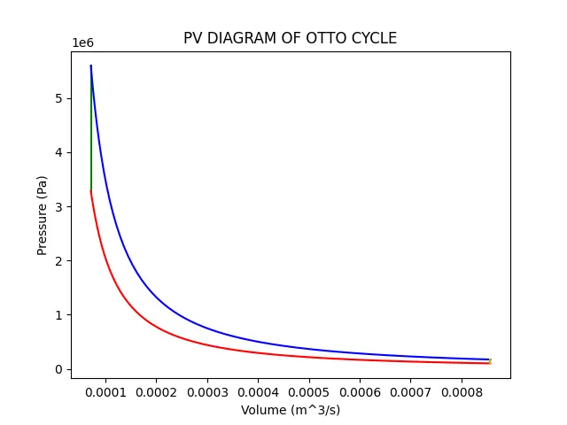
the diagram is plotted for better understanding of the otto cycle.
process one to three is given below.
#plotting of the pv diagram is done
plt.plot([v2,v3],[p2,p3],'g')
plt.plot(v_compression,p_compression,'r')
process three to back again to one is given below.
the plots and traces are given names and different colors fo easy identification.
plt.plot(v_expansion,p_expansion,'b')
plt.plot([v4,v1],[p4,p1],'y')
plt.title('PV DIAGRAM OF OTTO CYCLE')
plt.xlabel('Volume (m^3/s)')
plt.ylabel('Pressure (Pa)')
plt.show()
the thermal efficiency of the otto cycle is asked in the question for which the formula is stated here.
#thermal efficiency of the otto cycle
n = 1 - (pow(cr,(1-gamma)))
the value of thermal efficiency is printed out.
print(n)
PLOT:
THE THERMAL EFFICIENCY OF THE OTTO CYCLE:
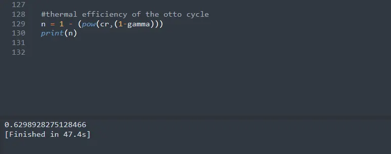
ηth = 0.6298
ERRORS:
1.there were some typos and colon operator error.
2.plt.show() was missing so the plot wasn't shown as output.
3.some indentation errors.
these errors are rectified with the help of the below popped command and the plotting of the otto cycle is done correctly.
conclusion:
the plotting of the pv diagram is done for the otto cycle and the thermal efficiency of the cycle is found.