Week 2 Air standard Cycle

Aim:

Writing a code that can solve an otto cycle and make plots for it.

The requirements are

1. Code should create a PV diagram

2. Output the thermal efficiency of the engine.

Theory:

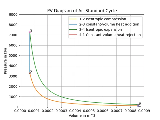
To write a program that plots the PV diagram of an otto cycle, we should first understand the PV diagram. The diagram plots the relationship between the pressure and the volume of the air-fuel mixture inside an IC engine at different stages during the otto cycle. the first stage is isentropic compression. This occurs during the compression stroke of the engine where the piston travels upwards towards the top dead centre (TDC) to compress the air-fuel mixture. Work is down by the piston on the air-fuel mixture to compress it. The second stage is called adiabatic heat addition. In this stage, no transfer of work or heat is done. This happens at constant volume. The third stage is called isentropic expansion. This occurs during the power stroke of the otto cycle where the piston travels downwards to the bottom dead centre (BDC) as work is done on it by the air-fuel mixture. The last stage is called adiabatic heat rejection. This also happens at constant volume.

The Otto cycle is the ideal cycle for spark-ignition reciprocating engines. It serves as the theoretical model for the gasoline engine:

• Consists of four internally reversible processes
• Heat is transferred to the working fluid at a constant volume

The Otto cycle consists of four internally reversible processes in series:

• 1-2 Isentropic compression
• 2-3 constant-volume heat addition
• 3-4 Isentropic expansion
• 4-1 Constant-volume heat rejection

Procedure:

All the explanation and defining variables are done along with the program.

Python Program:

# Program for Air Standard Cycle

# By Harshavardhana G

# Step-1: Importing modules
import math
import matplotlib.pyplot as plt
import numpy as np
import scipy as si

# The Otto cycle consists of the four process
# 1-2 Isentropic Compression or Reversible Adiabatic compression
# 2-3 Constant Volume Heat Addition
# 3-4 Isentropic Expansion or Reversible Adiabatic Expansion
# 4-1 Constant Volume Heat Rejection

# Terms in Otto Cycle

# Formula for Piston kinematics
# V/V_clearance = 1+0.5(cr-1)[R+1-cosd(theta)-(R^2-sind(theta))^0.5]
# Engine Geometry parameters
# Bore = 0.1m
# Stroke = 0.1m
# Connecting rod length (con_rod) = 0.15m
# Compression Ratio(cr) = (Vs+Vc)/(Vc)
# v1 = volume before compression = V_swept + V_clearance
# v2 = volume after compression = V_clearance
# V_s = V_swept = (pi/4)*Bore^2*Stroke
# V_c = V_clearance = V_s/(cr-1)
# cr = (V_s+V_c)/(V_c);
# Expanssion Ratio(er) = (v4)/(v3)
# er = v4/v3;

# defining the function of Engine Kinematics
def engine_kinematics(bore, stroke, con_rod, cr, start_crank, end_crank):

	a = stroke/2
	R = con_rod/a

	# Volume parameters
	V_s = math.pi*(1/4)*pow(bore,2)*stroke
	V_c = V_s/(cr-1)

	sc = math.radians(start_crank) 
	ec = math.radians(end_crank) 

	num_values = 50
	
	dtheta = (ec-sc)/(num_values-1)

	V = [] # creating array for volume values

	for i in range(0,num_values):
		theta = sc + i*dtheta
		term1 = 0.5*(cr-1)
		term2 = R + 1 - math.cos(theta)
		term3 = pow(R,2) - pow(math.sin(theta),2)
		term3 = pow(term3,0.5)

		V.append((1 + term1*(term2 - term3))*V_c)
	
	return V
# Input Variables
# State Variable at Point 1
p1 = 101.325 # in kPa
t1 = 500 # in K
gamma = 1.4
t3 = 3000 # in K

# Geometric Parameters
bore = 0.1
stroke = 0.1
con_rod = 0.15 
cr = 12

# Volume Computation of Swept volume and Clearance volume
v_s = (math.pi/4)*pow(bore,2)*stroke
v_c = v_s/(cr-1)
v1 = v_c + v_s

# State Variables at Point 2
v2 = v_c
# p2v2^gamma = p1v1^gamma
p2 = p1*pow(v1,gamma)/pow(v2,gamma)

# Due to isentropic compression, we can apply the PV Relation.
# p2v2/t2 = p1v1/t1 | rhs = p1v1/t1 | p2v2/t2 = rhs| t2 = p2v2/rhs
rhs = p1*v1/t1
t2 = p2*v2/rhs
V_compression = V = engine_kinematics(bore, stroke, con_rod, cr, 180,0)

constant = p1*pow(v1,gamma)
# P_compression*V_compression^gamma = constant

P_compression = []
for v in V_compression:
	P_compression.append(constant/pow(v,gamma))

# State Variables at Point 3
# Calculating Volume at point 3 (v3)
v3 =v2

# p3v3/t3 = p2v2/t2 | rhs = p2v2/t2 | p3 = rhs*t3/v3
rhs = p2*v2/t2
p3 = rhs*t3/v3

V_expansion = V = engine_kinematics(bore, stroke, con_rod, cr, 0,180)

constant = p3*pow(v3,gamma)
# P_expansion*V_expansion^gamma = constant

P_expansion = []
for v in V_expansion:
	P_expansion.append(constant/pow(v,gamma))

# State variables at Point 4
# Calculating Volume at point 4 (v4)
v4 = v1
#p4v4^gamma = p3v3^gamma
p4 = p3*pow(v3,gamma)/pow(v4,gamma)
# p4v4/t4 = rhs
t4 = p4*v4/rhs

# Thermal Efficiency of an Otto Cycle and its calculation
a = pow(cr,(gamma-1))
Thermal_Eff = (1 - pow(a,-1))*100
print('Thermal Efficiency of an Otto Engine =', Thermal_Eff,'%')

# Plotting
l2, = plt.plot([v2,v3],[p2,p3])
l1, = plt.plot(V_compression,P_compression)
l3, = plt.plot(V_expansion,P_expansion)
l4, = plt.plot([v4,v1],[p4,p1])
plt.plot(v1,p1,'*')
plt.plot(v2,p2,'*')
plt.plot(v3,p3,'*')
plt.plot(v4,p4,'*')
plt.text(0.0008607979964335801, 0, r'$	1   $')
plt.text(0.00007139983303613168, 3285.26, r'$	2   $')
plt.text(0.00007139983303613168, 7295.40, r'$	3   $')
plt.text(0.0008606797996433, 230, r'$	4    $')
plt.legend((l1,l2,l3,l4),['1-2 Isentropic compression','2-3 constant-volume heat addition','3-4 Isentropic expansion','4-1 Constant-volume heat rejection'])
plt.xlabel('Volume in m^3')
plt.ylabel('Pressure in kPa')
plt.title('PV Diagram of Air Standard Cycle')
plt.grid()
plt.xlim([0,0.0009]) # limiting the axis to 0.0009
plt.ylim([0,9000]) # limiting the axis to 9000
plt.savefig('PV Diagram for Air Std Cycle')
plt.show()

Result:

The thermal efficiency of an Otto engine = 62.98%

The below block shows the calculated thermal efficiency of the engine using codes.

Conclusion:

The desired and correct PV diagram of the Otto cycle was obtained using Python coding.

The output of the thermal efficiency of the engine is calculated.

Thank You...