Week 2 Air standard Cycle

Objective

Code to plot the P-V diagram in the otto cycle and calculate the efficiency of the otto cycle.

Solution Procedure

1. We need to import the math library, plot library for certain calculations and processes.

2. To plot the P-V diagram in the otto cycle and efficiency of the cycle some input values are required. We have to take the engine geometry parameters which are bore, stroke, length of the connecting rod, and the compression ratio. I have taken bore = 0.1, stroke = 0.1, connecting rod = 0.15, compression ratio = 12.

3. Now we are going to define a function to calculate the pressure and volume at the different-different crank angle to get the actual graph.

In the function, we can calculate how the volume is changing with respect to the change in the crank angle.

4. We are gonna need the value of gamma, pressure, and temperature at the starting of the compression (p1 & t1), the temperature at the start of the expansion(t3). I have taken gamma = 1.4, p1 =101325, t1 = 500, and t3 = 2300.

5.  Now we have to calculate the swept volume and clearance volume so that we can calculate the volume at state points 1 & 2.

swept volume = `pi/4*"bore"^2*stroke`

clearance volume = swept volume/(compression ratio-1)

6. Now we are going to calculate the variable at state point 2. The process from point 1 to 2 is the 'Isentropic Compression process'. We already have the value of v2. So we need to calculate the value of p2. We calculate the p2 value by "isentropic relation" that is `pv^gamma`= constant. Now to calculate the value of t2, we are going to use the "ideal gas law" which is pv/t = constant.

7. Now I am going to use the 'engine_kinematics' function to get the actual graph that occurs in the otto cycle. So that we can get the curve in the graph during the compression and expansion process. 

V_compression = engine_kinematics(bore,stroke,con_rod,cr,180,0)                                                       

The values of bore, stroke, con_rod, and cr are already given in the code. The value of the crank angle during the compression goes from 180 to 0.

We can calculate the combustion pressure with the help of the combustion volume.

P_compression = constant/V_compression^gamma

We are using the append command to store all the pressure and volume value at the different-different crank angle.

8. Now we are going to calculate the variable at state point 3. The process from point 2 to 3 is the 'constant volume heat addition process. The process is a constant volume process so v2 = v3. To get the value of p3 we are going to use the 'Ideal Gas Law' that is pv/t = constant.  

Again we are going to use the 'engine_kinematics' function. This time to calculate the expansion volume.

V_expansion= engine_kinematics(bore,stroke,con_rod,cr,0,180)

During the expansion process the angle of the crank goes from 0 to 180.

Now we can calculate the expansion pressure with the help of the expansion volume.

P_expansion = constant/V_expansion^gamma

9. Now we are going to calculate the variable at state point 4. The process from point 4 to 1 is the 'constant volume heat rejection process'. The process is a constant volume process so v4 = v1.  The process from point 3 to 4 is the 'Isentropic expansion process' We calculate the p4 value by "isentropic relation" that is pv^gamma= constant. Now to calculate the value of t4, we are going to use the 'ideal gas law' which is pv/t = constant.

10. Now we are going to calculate the thermal efficiency of the Otto cycle. 

thermal efficiency = `1-(t4-t1)/(t3-t2)`

11. Now we are going to plot the graph. For plotting the graph we are going to use plt.plot command. We are going to give the labels to both axes and the title of the graph.

Python Script

# Otto Cycle

import math
import matplotlib.pyplot as plt 

# Geometric Parameter
bore = 0.1
stroke = 0.1
con_rod = 0.15
cr = 12

def engine_kinematics(bore,stroke,con_rod,cr,start_crank,end_crank):
	# Geometric Parameter
	a = stroke/2
	R = con_rod/a

	# Volume Computation

	# Swept Volume
	v_s = (math.pi/4)*pow(bore,2)*stroke

	# Clearence Volume
	v_c = v_s/(cr-1)

	# Starting Crank angle
	sc = math.radians(start_crank)
	# Ending Crank angle
	ec = math.radians(end_crank)

	num_values = 100

	dtheta = (ec-sc)/(num_values-1)
	V = []

	for i in range(0,num_values):
		theta = sc + i*dtheta
		term1 = 0.5*(cr-1)
		term2 = R + 1 - math.cos(theta)
		term3 = pow(pow(R,2) + pow(math.sin(theta),2),0.5)

		V.append((1 + term1*(term2-term3))*v_c)

	return V


# Inputs
p1 = 101325
t1 = 500
gamma = 1.4
t3 = 2300

# Volume Computation

# Swept Volume
v_s = (math.pi/4)*pow(bore,2)*stroke

# Clearence Volume
v_c = v_s/(cr-1)

# State Point 1
v1 = v_c + v_s

# State point 2
v2 = v_c

# Process 1-2 is Isentropic Heat Rejection Process
# p1v1^(gamma) = p2v2(gamma)
p2 = (p1*pow(v1,gamma))/pow(v2,gamma)

# p1*v1/t1 = p2*v2/t2
rhs = p1*v1/t1
t2 = p2*v2/rhs
V_compression = engine_kinematics(bore,stroke,con_rod,cr,180,0)

constant = p1*pow(v1,gamma)
P_compression = []

for v in V_compression:
	P_compression.append(constant/pow(v, gamma))



# State Point 3
v3 = v2

# p3*v3/t3 = p2*v2/t2
rhs = p2*v2/t2
p3 = rhs*t3/v3

V_expansion = engine_kinematics(bore,stroke,con_rod,cr,0,180)

constant = p3*pow(v3,gamma)
P_expansion = []

for v in V_expansion:
	P_expansion.append(constant/pow(v, gamma))


# State 4
v4 = v1 

# Process 3-4 is Isentropic Heat Addition Process
# p3v3^(gamma) = p4v4^gamma)
p4 = (p3*pow(v3,gamma))/pow(v4,gamma)

# p3*v3/t3 = p4*v4/t4
rhs = p3*v3/t3
t4 = p4*v4/rhs

thermal_efficiency = 1-(t4-t1)/(t3-t2)
print(thermal_efficiency)

plt.plot([v2,v3],[p2,p3])
plt.plot([v4,v1],[p4,p1])
plt.plot(V_compression, P_compression)
plt.plot(V_expansion, P_expansion)
plt.xlabel('Volume')
plt.ylabel('Pressure')
plt.title('Otto Cycle')
plt.show()

Output

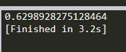
After running the program we get the efficiency value = 0.62989 

The plot we get by executing this code is as following:-

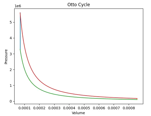
We can see from the above graph. Process 1 to 2 is isentropic compression process. Which we can see in the plot as a green color curve. Process 2 to 3 is the constant volume heat addition process. Which we can see in the plot as the blue line. Process 3 to 4 is the isentropic expansion process. Which we can see in the plot as a red color curve. Process 3 to 4 is the constant volume heat rejection process. Which we can see in the plot as an orange line.