Week 2 Air standard Cycle

AIM:

• Using forward kinematics concepts construct the PV diagram of Otto cycle of an engine for a given set of dimensions.
• Also find the Thermal efficiency of the engine.

Governing equations:

Sweptvolume=`pi/4*B^2*S`

Clearance volume=`(sweptvolume)/(C.R-1)`

Relation between volume and crank angle is:

`V/V_c=1+(C.R-1)/2[R+1-costheta-(R^2-sin^2theta)^(1/2)]`

here

B=Bore of the engine(m)

S=stroke of the engine(m)

`theta`=crank angle(degrees)

C.R=compresson ratio

`V_c`=cleaarance volume

R=`2*(l/S)`(where l is length of connecting rod of engine)

relations used to calculate pressure,volume temparature at statepoints are:

`P_1V_1^gamma=P_2V_2^gamma`

`P_3V_3^gamma=P_4V_4^gamma`

`(P_1*V_1)/T_1=(P_2*V_2)/T_2`

`(P_2*V_2)/T_2=(P_3*V_3)/T_3`

`(P_3*V_3)/T_3=(P_4*V_4)/T_4`

`V_3=V_2`

`V_4=V_1`

`V_1=sweptvolume+clearance volume`

`V_2=clearance volume`

above are relations between pressure, volume ,temparature at state points 1,2,3,4`

thermal efficiency of engine=`1-1/(C.R^(gamma-1))`

gamma=ratio of specific heats of the gas

Theory:

• Otto cycle demonstrates about what happens to a gas when it is subjected to a change in temparature,pressure and volume as well as addtion and removal of heat. when it is kept in a cylinder.
• Here,we considered an engine for observing the changes in gas.

Here ,TDC is top dead centre and BDC is bottom dead centre of the cylinder.

Procedure:

• Inorder to generate the PV diagram,we need a set of values of volumes in the adiabatic regions.Fot that we need values of volume for every crank angle.This helps us in getting the curved path.
• So inorder to get volume values for every crank angle a program is written for that .it is shown below:

import math
import numpy as np
#function for generating volumes for different crank angles
def engine_kinematics(bore,stroke,con_rod,CR,start_crank,end_crank):
    bore=0.10
    stroke=0.1
    con_rod=0.15
    CR=12
    a=stroke/2
    R=con_rod/a
    V_s=math.pi/4*pow(bore,2)*stroke
    V_c=V_s/(CR-1)
#crank angles are taken as dtheta
    sc=math.radians(start_crank)
    ec=math.radians(end_crank)
    num_values=50
    dtheta=(ec-sc)/(num_values-1)
    v=[]
    for i in range(0,num_values):
        theta=sc+i*dtheta
        term1=0.5*(CR-1)
        term2=R+1-math.cos(theta)
        term3=pow(R,2)-pow(math.sin(theta),2)
        term4=pow(term3,0.5)
        v.append((1+term1*(term2-term4))*V_c)
    return v

• Here, a function is created for generating volumes for every crankangle varying from 0 to 180.
• The function named as "engine knematics is created with arguments as values of bore,stroke,length of connecting rod,compressionratio,and as well as starting and ending crankangle.
• Considering the formula i.e which is the relation between volume and crankangle ,for simple calculation , the formula is divided into terms and each term is evaluated seperatley so that at the end we can add all of them to get the answer.
• these all values are appended by using append command and stored in the array.
• The return values of this function is an array of values of volume for a given set of specifications of engine.

For the pv diagram construction ,the code is given below:

import math
import matplotlib.pyplot as plt
import numpy as np
#pressure
p1=101325
#temparatures
t1=500
t3=2300
gamma=1.4
#dimensions of engine
bore=0.1
stroke=0.1
con_rod=0.15
CR=12
#sweptvolume
v_s=(math.pi/4)*pow(bore,2)*stroke
v_c=v_s/(CR-1)
v1=v_c+v_s
#state point2
v2=v_c
p2=p1*pow(v1,gamma)/pow(v2,gamma)
#calculate t2
lhs=(p1*v1)/t1
t2=(p2*v2)/lhs
v_compression=engine_kinematics(bore,stroke,con_rod,CR,180,0)
constant=p1*pow(v1,gamma)
p_compression=[]
for v in v_compression:
    p_compression.append(constant/pow(v,gamma))
#state point3
v3=v2
rhs=(p2*v2)/t2
p3=rhs*t3/v3
v_expansion=engine_kinematics(bore,stroke,con_rod,CR,0,180)
constant=p3*pow(v3,gamma)
p_expansion=[]
for v in v_expansion:
    p_expansion.append(constant/pow(v,gamma))
#state point4
v4=v1
p4=p3*pow(v3,gamma)/pow(v4,gamma)
t4=p4*v4/lhs
#plotting otto cycle
plt.plot([v2,v3],[p2,p3],label='heat addition')
plt.plot(v_compression,p_compression,label='compression')
plt.plot(v_expansion,p_expansion,label='expansion')
plt.plot([v4,v1],[p4,p1],label='heat rejected')
plt.legend(['heat addition','compression','expansion','heat rejection'],loc="upper right")
plt.savefig("ottocycle.png")
#thermal efficiency
Th_ef=(1-1/(pow(CR,(gamma-1))))*100
print("thermalefficiency is:")
print(Th_ef)

• In this code first of all specifiations of enigne is given as input by creating variables for them.
• As well as the initial pressure,temparature,and gamma values of the gas is also declared as variables and values are initialised for them.
• Now , we calculate volume at the first point by calcualting clearence volume and swept volume of the engine by formulas mentioned above.
• After obtaining the volume at state point1,then by using relation mentioned in the formulas above we calculate pressure and Temparature at state point2
• For the compression region the function we created above is called here.In that arguments , the starting and ending crank angles are given as 0,180 .Using a for loop ,the pressure values in compression region are thus calculated for every volume and stored in the array.
• From state point 3 to 4 its expansion so again function is called but this time the crank angle varies from 180 to 0.Using forloop ,the pressure values of expansion region are calculated and stored in the array.
• As well the pressure , volume, temparature of statepoint 4 are also calculated using relations mentioned above.
• Then a graph is plotted by plotting the pressure , volume values obtained at all the state point and as well as the values of pressure andvolume in compression and expansion region is also plotted .
• using matplotlib library and legend command the whole region is labelled in detail.

The P-V graph obtained by considering the above values is shown below:

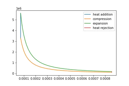
• And at last the thermal efficiency of the engine is also calculated by using the formual mentioned above.
• The thermal efficiency obtained by using the values mentioned above is :62.98928275128466%

Conclusion:

• Thus P-V diagram of ottocycle is plotted using the concepts of forward kinematics and principles of thermodynamics and thermal efficinecy of the engine is obtained