Week 3 - Solving second order ODEs

AIM:

• Solve the second order ODe equation of pendulum with damping constants for the given specifications of the pendulum.
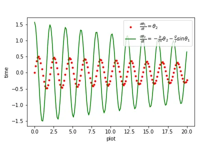
• Plot the wave of the angular displacement and as well as angular velocity.
• show the animation of the pendulum oscillating according to given constraints.

Theory:

The second order differential equation of motion of a simple pendulum with damping. is defined as:

`(d^2theta)/dt^2+(b/m)(d theta)/dt+g/lsintheta=0`

In the above equation,

g = gravity in m/s2,

L = length of the pendulum in m,

m = mass of the ball in kg,

b=damping coefficient.

Procedure:

• The given equation is a sewcond order ODE.In order to olve it in python we need to first convert it into a first order ODE so that we can use ODe solver in python to solve it.

So first of all consider `theta=theta_1`

subsituting it in ODE we get:

`(d^2theta_1)/dt^2+(b/m)(d theta_1)/dt+g/lsintheta_1=0`

Let `(d theta_1)/dt=theta_2`--------(1)

then `(d^2theta_1)/dt^2=(d theta_2)/dt`,substitute this value we get,

`(d theta_2)/dt+(b/m)(theta_2)+g/lsintheta_1=0`

`(d theta_2)/dt=-(b/m)(theta_2)-g/lsintheta_1`-------------(2)

The equation (1) and (2) are considered for solving using the ode solver

Here is the code written for solving the ODE:

import numpy as np
from scipy.integrate import odeint
import matplotlib.pyplot as plt
import math
theta=[]
#function that returns dtheta/dt
def model(theta,t,b,g,l,m):
    theta1=theta[0]
    theta2=theta[1]
    dtheta1_dt=theta2
    dtheta2_dt=-(b/m)*theta2-(g/l)*math.sin(theta1)
    dtheta_dt=[dtheta1_dt,dtheta2_dt]
    return dtheta_dt
#arguments to be given
b=0.05
g=9.81
l=1
m=1
#initial condition
theta_0=[0,math.pi/2]
#time points
t=np.linspace(0,20,150) 
#ode solving
theta= odeint(model,theta_0,t,args=(b,g,l,m))

#plotting results
plt.plot(t,theta[:,0],'r.',label=r'$\frac{d\theta_1}{dt}=\theta_2$')
plt.plot(t,theta[:,1],'g-',label=r'$\frac{d\theta_2}{dt}=-\frac{b}{m}\theta_2-\frac{g}{l}sin\theta_1$')
plt.legend(loc="best")
plt.xlabel('plot')
plt.ylabel("time")
plt.savefig("pendulum")
#For simulating the pendulum
theta_x1=0
t_x=theta[:,0]
ct=0
for i in range(0,150):
    filename=str(ct) + '.png'
    ct=ct+1
    plt.figure()
    plt.plot([0,1],[theta_x1,t_x[i]],marker='o',markersize='25')
    plt.xlim([-1.5,1.5]) 
    plt.ylim([-1.5,1.5])
    plt.savefig(filename)
    

• first of all we created a function for the differential equations which we have obtained above.This function is given arguments of dampingconstant,length of pendulum,mass of pendulum,gravity.
• Inorder to solve ODE we import odeint module from scipy library.
• And inorder for giving arguments , the values of length, mass,damping constant are declared.
• As well as for solving the ODE,time points and displacement conditons are also declared and initialised.
• Then using odeint the theta values are obtained,by feeding the module with the function declared above, the arguments required and as well as the initial conditions declared.
• The solutions obtained are plotted on the graph with time to obtain the wave form of angular displacement and angular velocity.

The graph obtained is shown below:

• Now for the animation, we have plotted the angular displacement values obtained form the ODE solution and the plotted the position for every angular displacement.
• For that the array obtained from the ODE solver , we consider the whole first column values and used for the plot.

The video of animation of the position of the pendulum is given below:

https://youtu.be/uRA7LBR6SlQ

Conclusion:

• Thus the second order ODE of the pendulum with damping is solved using relevant ODEsolver in python.
• The wave form of angular displacement and angular velocity is obtained and displayed.
• The animation of the pendulum from the solutions obtained from theODe is demonstrated.