Week 5 - Curve fitting

Aim:

• To write a code to fit a linear and cubic polynomial for the given datset comprising of values of temparature and specific heat at constant pressure.
• Show emperically as how the curve has fit.
• Plot all the curves obtained.
• Explain the reasons and process used for choosing best fit.

Theory:

Curve fitting is the process of plotting acurve for a givemn mathematical function which has the best fit to the series of original values of the given dataset.

In other terms, weplot 2 curves one from the datset values and the otherfromthe values obtained from the considered function and calculate accuracy between original and calculated values.

Formulas used :

sum of squares of errors(sse)=`sum(Observed value - predicted value)^2`

sum of squares due to regression(ssr)=`sum(predicted values-mean of the observed values)^2`

sum of squares total(sst)=sse+ssr

Measure of goodness of fit (`R^2`)=sst/ssr

Procedure:

• The below code is the one written for curve fitting

import math
import numpy as np
import matplotlib.pyplot as plt
from scipy.optimize import curve_fit
#curve fit functions
def func_0(t,a,b):
    return a*t+b
def func_1(t,a,b,c):
    return a*pow(t,2)+b*t+c
def func_2(t,a,b,c,d):
    return a*pow(t,3)+b*pow(t,2)+c*t+d
#reading thermodynamic datafile
def read_file():
    temparature=[]
    cp=[]
    for line in open('data','r'):
            values=line.split(',')
            temparature.append(float(values[0]))
            cp.append(float(values[1]))
    return [temparature,cp]
temparature,cp=read_file()
# curve fitting for linear fit
popt_0,pcov_0=curve_fit(func_0,temparature,cp)
fit_cp=func_0(np.array(temparature),*popt_0)
plt.plot(temparature,cp,color="blue")
plt.plot(temparature,fit_cp,color='red')
plt.title('linear curve fitting')
plt.legend(['Actualcurvefit','curvefit'])
plt.xlabel('temparature')
plt.ylabel('cp')
plt.savefig('linear fit')
#calculating Rsquare value for linear fit
sum_cp=np.sum(cp)
size_cp=np.size(cp)
mean_cp=sum_cp/size_cp
sse_0=0
err_0=0
ssr_0=0
sst_0=0
for i in range(size_cp):
    err_0=(cp[i]-fit_cp[i])
    sse_0=sse_0+pow(err_0,2)
    ssr_0=ssr_0+pow((fit_cp[i]-mean_cp),2)
sst_0=sse_0+ssr_0
Rsquare_0=ssr_0/sst_0
print('Rsquare value for linear fit:')
print(Rsquare_0)
#curve fitting for quadratic fit
popt_1,pcov_1=curve_fit(func_1,temparature,cp)
fit_cp1=func_1(np.array(temparature),*popt_1)
plt.figure(2)
plt.plot(temparature,cp,color="blue")
plt.plot(temparature,fit_cp1,color='red')
plt.title('quadratic curve fitting')
plt.legend(['Actualcurvefit','curvefit'])
plt.xlabel('temparature')
plt.ylabel('cp')
plt.savefig('quadratic fit')
#calculating Rsquare value for cubicfit
sse_1=0
err_1=0
ssr_1=0
sst_1=0
for i in range(size_cp):
    err_1=(cp[i]-fit_cp1[i])
    sse_1=sse_1+pow(err_1,2)
    ssr_1=ssr_1+pow((fit_cp1[i]-mean_cp),2)
sst_1=sse_1+ssr_1
Rsquare_1=ssr_1/sst_1
print('Rsquare value for quadratic  fit:')
print(Rsquare_1)
#curve fitting for cubic fit
popt_2,pcov_2=curve_fit(func_2,temparature,cp)
fit_cp2=func_2(np.array(temparature),*popt_2)
plt.figure(3)
plt.plot(temparature,cp,color="blue")
plt.plot(temparature,fit_cp2,color='red')
plt.title('cubic curve fitting')
plt.legend(['Actualcurvefit','curvefit'])
plt.xlabel('temparature')
plt.ylabel('cp')
plt.savefig('cubic fit')
#calculating Rsquare value for cubic fit
sse_2=0
err_2=0
ssr_2=0
sst_2=0
for i in range(size_cp):
    err_2=(cp[i]-fit_cp2[i])
    sse_2=sse_2+pow(err_2,2)
    ssr_2=ssr_2+pow((fit_cp2[i]-mean_cp),2)
    
sst_2=sse_2+ssr_2
Rsquare_2=ssr_2/sst_2
print('Rsquare value for cubic fit:')
print(Rsquare_2)

• In this code we first create 3 functions fro linear,quadratic and as well as cubic polynmial with arguments as temparature,a,b,c.
• Then we import the dataset and open the file.using split command we split the dataset imported and append all the temparature and specific heat values seperately in 2 arrays seperately.
• Now for curve fitting in python we use curve fit module which can be obtained by importing scipy library.
• So by using curve fit module we calculate the coefficients and covariances for the given equaions one by one seperately.

Common queries arised from the code:

1.What does popt and pcov mean in the above code?

A:popt is an array consisting of optimum values of the coefficients for which the sum of squares of residuals is minimised.

pcov is is basically a multidimensional array created with the values obtained by estimating the covariance obtained from the above values of popt i.e coefficients.we take diagonal elements in the array as the varinace of each parameter in popt.the dimension of array depends on no of coefficients.

2.What does np.array(temperature) do?

A:It creates an array with the values of temaprature by maintaining same type and inexing them with a tuple of non-negative integers.

3.What does the *popt mean?

A:It is used to call the best fit pararmeters calculated from the curve fit method into the function we declared above i.e the equations.'*' notation will exapnd them into arguments of the function.

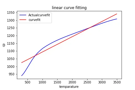
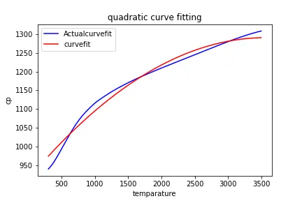
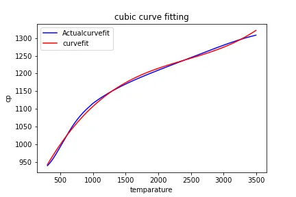
• Now going into the code , we then plot 2 graphs taking temparature as X-axis and specific heat as Y-axis ,one from the values we have from the dataset and the other values obtained by using the curve fit method.

The graph of linear fit is given below:

The graph of quadratic fit is given below:

The graph of cubic fit is given below:

Now for measuring the goodnes of fit we need the `R^2` value for that.

• So, i have written a code using the formulas mentioned above and calculated `R^2` value for every curve fit

`R^2` value for linear fit:
0.9248776260524184

`R^2` value for quadratic  fit:
0.9812421444745516

`R^2`value for cubic fit:
0.996725946714689

What needs to be done in order to make the curve fit perfect?

A:method1: By chaging the order of the polynomial, we can try to get best fit at any state.

method2:By using splitwise curve fit i.e by splitting the data set into small sets and finding the best fits for them.in this method we can get best fit may be in lower order polynomials itself.

How to show empirically as to how well your curve has been fit?

A:Basically we consider the goodness of fit value for that.

if `R^2`=1 then curve is perfectly fit

if `R^2`<0.5 then curve is badly fit

if `R^2` is inbetween 0.98 and 0.99 then the curve is best fit

More `R^2` value ,the more likely the curve is considered as best fit.

Conclusion:

• By considering the `R^2` values of linear,quadratic and cubic fits we observe that cubic fit as good value.
• For more accurate fits we can also go for higher order polynomials for fitting or use splitwise fitting method.