Validation studies of Symmetry BC vs Wedge BC in OpenFOAM vs Analytical H.P equation

Expected Results

1. Validate Hydro-dynamic length with the numerical result
2. Validate the fully developed flow velocity profile with its analytical profile
3. Validate maximum velocity and pressure drop for fully developed flow
4. Post-process Shear stress and validate wall shear stress for fully developed flow
5. Highlight the differences in both boundary conditions in terms of their usage and application.

Angles to test:

• 10
• 25
• 45

For a circular pipe, the flow becomes turbulent after when Reynold's number becomes greater than 4000 and in between 2300-4000 the flow remains in the transition state.

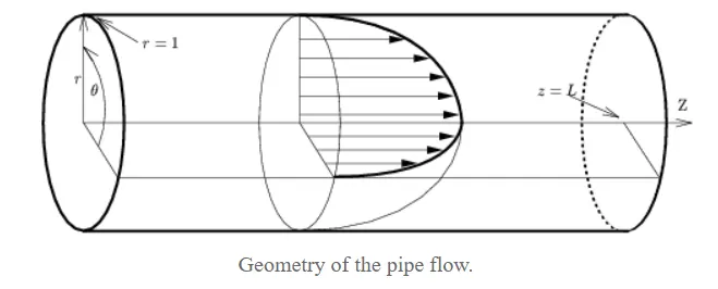
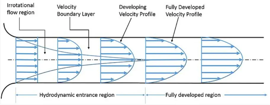
At the entrance, the flow is said to be in the hydrodynamic entrance region where the velocity profile gradually takes the shape of a parabola from a straight line. As soon as the parabolic velocity profile becomes steady the flow is said to be in its fully developed state. Normally Hagen Poiseuille's Equation is applicable for fully developed flow which helps us to calculate the pressure loss. The distance required for a flow to develop is called the entrance length(Le), and depends on the shear stresses that act on the pipe wall.

For a circular pipe, we can calculate the average and maximum velocity, maximum shear stress and pressure loss analytically which are as follows.

`underset(avg)(v)=(muRe)/(rho underset(h)(D)`

`underset(max)(v)=2 underset(avg)(v)`

`underset(max)(tau)=(2muv)/(underset(h)(r))`

pressure drop=`DeltaP=(32mu underset(avg)(v)(L-Le))/(underset(h)(D)^2)`

here,

`underset(h)(D)`=Diameter

Entry Length=`underset(e)(L)=0.06*Re*underset(h)(D)`

Length of pipe=L=`0.05+underset(e)(L)`

Kinematic pressure=`(DeltaP)/(rho)`

sheer stress=`tau=-mu(du)/(dy)`

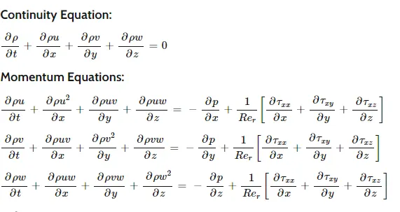
Governing equations

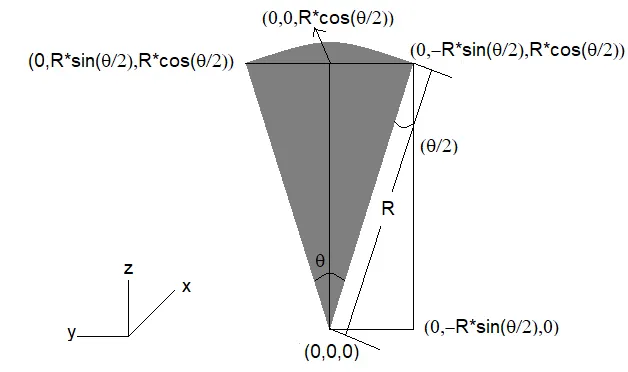
Pipe Geometry

For pipe flow applications, it’s often important to be able to determine whether a given flow condition is laminar flow or turbulent flow. Different equations or methods of analysis often apply to laminar flow and turbulent flow conditions.The typical criterion for whether pipe flow is laminar or turbulent is the value of the Reynolds Number.

The Reynolds number for pipe flow is defined as

`Re=DVρ/μ = uL/ν` where

D is the pipe diameter,

V is the average flow velocity in the pipe,

ρ is the density of the flowing fluid and

μ is the dynamic viscosity of the flowing fluid.

`nu` is the kinematic viscosity =`ρ/μ`=`1/nu`.

Re is a dimensionless number.

Any consistent set of units can be used for D, V, ρ, and, will result in Reynolds number being dimensionless. The generally accepted criteria for laminar flow and turbulent flow in terms of Re are as follows:

For Re < 2100, it is laminar flow.

For Re > 4000, it is turbulent flow.

For 2100 < Re < 4000, the flow is in the transition region.

For flow in the transition region, the flow may be either laminar or turbulent, depending upon the nature of the entrance to the pipe and the pipe wall roughness.

A pressure drop between the beginning and the end of a pipe is the drive for a flow. However, the pressure gradient that forms over the length of the pipe has two tasks, so to speak. The pressure drop must not only compensate for the frictional force during the flow of the fluid but must accelerate the fluid to achieve the characteristic flow profile in the first place.

Therefore, the total pressure drop can be divided into a part that is used to accelerate the fluid and a part that is used to compensate for friction. In the above equations, the pressure gradient dp/dx only refers to that part of the total pressure gradient which is necessary to overcome the friction.

To determine this pressure gradient, one must not simply take the pressure difference between the beginning and end of the pipe and then divide it by the length of the pipe. This is why the above equations always referred to a pipe section where it was implicitly assumed that the parabolic flow profile had already been fully established.

The equation of Hagen-Poiseuille does not apply in the inlet of a pipe (inlet flow), within which the pressure gradient must accelerate the fluid to the typical parabolic profile in addition to overcoming friction.

Under certain circumstances, it may nevertheless be justified to describe flow by simply determining the pressure gradient in the above equations from the quotient of pressure drop and pipe length. Namely, whenever the work of acceleration is negligible compared to the friction work. This will always be the case if the pipe is relatively long compared to its diameter, or if the flow velocities are relatively low. In such cases, the frictional work usually clearly outweighs the relatively low work of acceleration due to the long pipe length.

function haagen(r,L,theta)
%% creating blockmesh dict file%% Opening Part
h1='/*--------------------------------*- C++ -*----------------------------------*';
h2='  =========                |';
h3='  \      / F ield         | OpenFOAM: The Open Source CFD Toolbox';
h4='   \    /  O peration     | Website: https://openfoam.org';
h5='    \  /   A nd           | Version: 9';
h6='     \/    M anipulation  |';
h7='*---------------------------------------------------------------------------*/';
h8='FoamFile';
h9='{';
h10='    format      ascii;';
h11='    class       dictionary;';
h12='    object      blockMeshDict;';
h13='}';
h14='// * * * * * * * * * * * * * * * * * * * * * * * * * * * * * * * * * * * * * //';
f1=fopen('blockMeshDict.txt','wt');
fprintf(f1,'%sn',h1);
fprintf(f1,'%sn',h2);
fprintf(f1,'%sn',h3);
fprintf(f1,'%sn',h4);
fprintf(f1,'%sn',h5);
fprintf(f1,'%sn',h6);
fprintf(f1,'%sn',h7);
fprintf(f1,'%sn',h8);
fprintf(f1,'%sn',h9);
fprintf(f1,'%sn',h10);
fprintf(f1,'%sn',h11);
fprintf(f1,'%sn',h12);
fprintf(f1,'%sn',h13);
fprintf(f1,'%sn',h14);
%%vertices
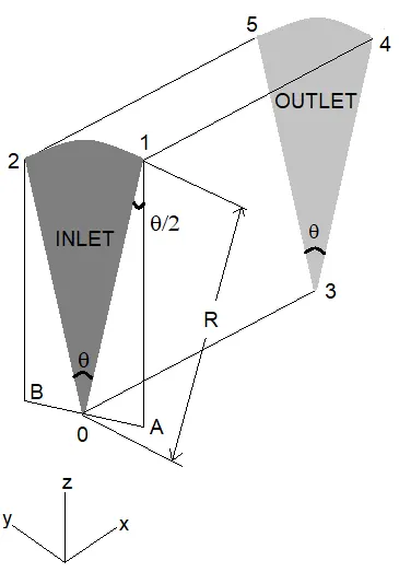
v0 = [0 0 0];
v1 = [0 r*cosd(theta/2) r*sind(theta/2)];
v2 =[0 r*cosd(theta/2) -r*sind(theta/2)];
v3 = [L 0 0];
v4 = [L r*cosd(theta/2) r*sind(theta/2)];
v5 = [L r*cosd(theta/2) -r*sind(theta/2)];
mid1 = [0 r 0];
mid2 = [L r 0];
%%Write vertices
h15='convertToMeters 1;';
fprintf(f1,'%snn',h15);
h16='vertices';
fprintf(f1,'%sn',h16);
h17='(';fprintf(f1,'%sn',h17);
fprintf(f1,'t(%d %d %d)n',v0);
fprintf(f1,'t(%d %d %d)n',v1);
fprintf(f1,'t(%d %d %d)n',v2);
fprintf(f1,'t(%d %d %d)n',v3);
fprintf(f1,'t(%d %d %d)n',v4);
fprintf(f1,'t(%d %d %d)n',v5);h18=');';
fprintf(f1,'%sn',h18);
%% write Blocks
h19='blocks';
h20='(';
if theta==10
h21=' hex (0 3 5 2 0 3 4 1) (500 25 2) simpleGrading (1 0.2 1)';
elseif theta==25
h21=' hex (0 3 5 2 0 3 4 1) (500 25 3) simpleGrading (1 0.2 1)';
elseif theta==50
h21=' hex (0 3 5 2 0 3 4 1) (500 25 3) simpleGrading (1 0.2 1)';
elseif theta<5
h21=' hex (0 3 5 2 0 3 4 1) (500 25 1) simpleGrading (1 0.2 1)';
end   
h22=');';
fprintf(f1,'n%sn',h19);
fprintf(f1,'%sn',h20);
fprintf(f1,'n%sn',h21);
fprintf(f1,'%sn',h22);
%% write edges
h23='edges';
h24='(';
h25=' arc 1 2';
h26=' arc 4 5';
h27=');';
fprintf(f1,'n%sn',h23);
fprintf(f1,'%sn',h24);
fprintf(f1,'%s (%d %d %d)n',h25,0, r, 0);
fprintf(f1,'%s (%d %d %d)n',h26,L, r, 0);
fprintf(f1,'%sn',h27);
%% write boundary 
inlet = [0 1 2 0];
outlet=[3 5 4 3];
surface=[2 1 4 5];
axis=[0 3 3 0];
front=[0 3 4 1];
back=[0 2 5 3];
fprintf(f1,'n%sn','boundary');
fprintf(f1,'%sn','(');
%inlet patch
fprintf(f1,'t%sn','inlet');
fprintf(f1,'t%sn','{');
fprintf(f1,'tt%sn','type patch;');
fprintf(f1,'tt%sn','faces');
fprintf(f1,'tt%sn','(');
fprintf(f1,'ttt(%d %d %d %d)n',inlet);
fprintf(f1,'tt%sn',');');
fprintf(f1,'t%sn','}');
%outlet patch
fprintf(f1,'nt%sn','outlet');
fprintf(f1,'t%sn','{');
fprintf(f1,'tt%sn','type patch;');
fprintf(f1,'tt%sn','faces');
fprintf(f1,'tt%sn','(');
fprintf(f1,'ttt(%d %d %d %d)n',outlet);
fprintf(f1,'tt%sn',');');
fprintf(f1,'t%sn','}');
%surface
fprintf(f1,'nt%sn','surface');
fprintf(f1,'t%sn','{');
fprintf(f1,'tt%sn','type wall;');
fprintf(f1,'tt%sn','faces');
fprintf(f1,'tt%sn','(');
fprintf(f1,'ttt(%d %d %d %d)n',surface);
fprintf(f1,'tt%sn',');');
fprintf(f1,'t%sn','}');
%axis
fprintf(f1,'nt%sn','axis');
fprintf(f1,'t%sn','{');
fprintf(f1,'tt%sn','type empty;');
fprintf(f1,'tt%sn','faces');
fprintf(f1,'tt%sn','(');
fprintf(f1,'ttt(%d %d %d %d)n',axis);
fprintf(f1,'tt%sn',');');
fprintf(f1,'nt%sn','}');
%front
fprintf(f1,'nt%sn','front');
fprintf(f1,'t%sn','{');
fprintf(f1,'tt%sn','type wedge; //symmetry');
fprintf(f1,'tt%sn','faces');
fprintf(f1,'tt%sn','(');
fprintf(f1,'ttt(%d %d %d %d)n',front);
fprintf(f1,'tt%sn',');');
fprintf(f1,'t%sn','}');
%back
fprintf(f1,'nt%sn','back');
fprintf(f1,'t%sn','{');
fprintf(f1,'tt%sn','type wedge; //symmetry');
fprintf(f1,'tt%sn','faces');
fprintf(f1,'tt%sn','(');
fprintf(f1,'ttt(%d %d %d %d)n',back);
fprintf(f1,'tt%sn',');');
fprintf(f1,'t%sn','}');
fprintf(f1,'%sn',');');
fprintf(f1,'n%sn','mergePatchPairs');
fprintf(f1,'%sn','(');
fprintf(f1,'%sn',');');
fprintf(f1,'n%sn','// ************************************************************************* //');
end

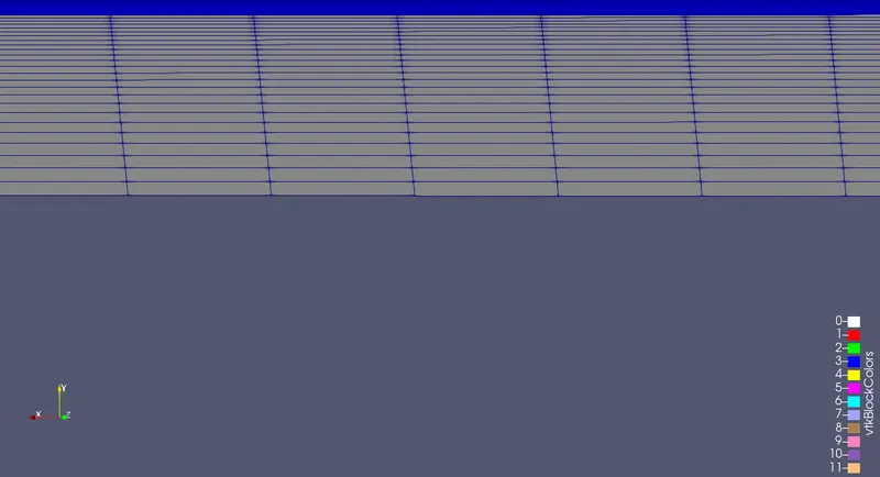
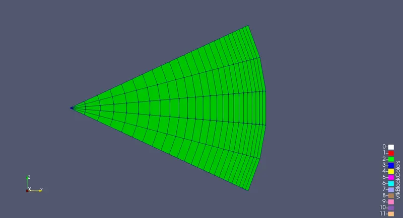
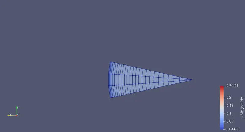
mesh in the crossectional area depends on the angle made by the arc and front & back can be changed simply in code.

Initial conditions

velocity=0.1476m/s

pressure=0 Pa

Fluid properties

`mu=8.9256e-07`

Runtime

Start time=0

End time =15.81

`DeltaT=0.058`

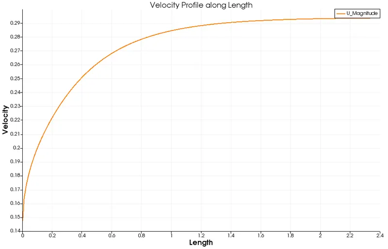
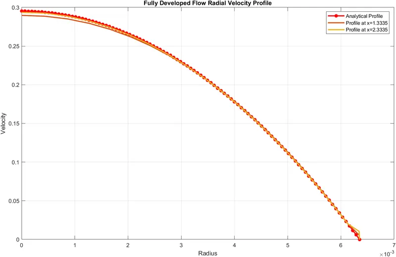
It is seen that after the hydrodynamic length the velocity along the length becomes constant. The same can be seen in the below which compares the Radial Velocity profile of Fully Developed Flow Profiles.

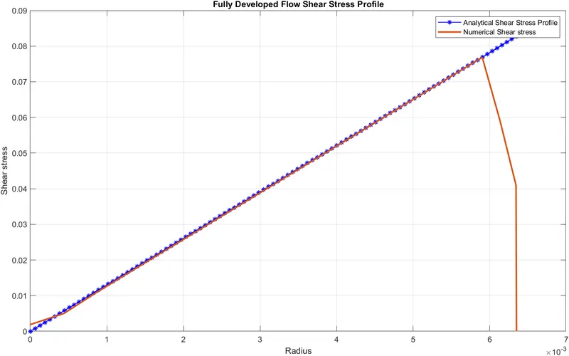
The shear stress at the pipe wall is related to the slope of the velocity `tau` profile at the surface. Noting that the velocity profile remains unchanged in the hydrodynamically fully developed region, the wall shear stress also remains constant.

The wall shear stress is the highest at the pipe inlet where the thickness of the boundary layer is smallest and decreases gradually to the fully developed value. Therefore, the pressure drop is higher in the entrance regions of a pipe and the effect of the entrance region is always to increase the average friction factor for the entire pipe.

figure(2)
plot(R,tau,'b*-','LineWidth',1)
hold on
tau_23335=readmatrix('Tau_2.3335.csv');
plot(tau_23335(:,1),tau_23335(:,2),'LineWidth',2)
xlabel('Radius')
ylabel('Shear stress')
grid on
legend ('Analytical Shear Stress Profile','Numerical Shear stress')
title('Fully Developed Flow Shear Stress Profile')
%Velocity Profile
figure(3)
plot(R,u,'r*-','LineWidth',2)
hold on
v_13335=readmatrix('U_x13335.csv');
v_23335=readmatrix('U_x23335.csv');
plot(v_13335(:,1),v_13335(:,2),'LineWidth',2)
plot(v_23335(:,1),v_23335(:,2),'LineWidth',2)
legend('Analytical Profile','Profile at x=1.3335','Profile at x=2.3335');
xlabel('Radius')
ylabel('Velocity')
title('Fully Developed Flow Radial Velocity Profile')
grid on

BlockMesh Dict

/*--------------------------------*- C++ -*----------------------------------*
  =========                |
  \      / F ield         | OpenFOAM: The Open Source CFD Toolbox
   \    /  O peration     | Website: https://openfoam.org
    \  /   A nd           | Version: 9
     \/    M anipulation  |
*---------------------------------------------------------------------------*/
FoamFile
{
    format      ascii;
    class       dictionary;
    object      blockMeshDict;
}
// * * * * * * * * * * * * * * * * * * * * * * * * * * * * * * * * * * * * * //
convertToMeters 1;

vertices
(
	(0 0 0)
	(0 5.755054e-03 2.683626e-03)
	(0 5.755054e-03 -2.683626e-03)
	(2.333500e+00 0 0)
	(2.333500e+00 5.755054e-03 2.683626e-03)
	(2.333500e+00 5.755054e-03 -2.683626e-03)
);

blocks
(

 hex (0 3 5 2 0 3 4 1) (500 25 5) simpleGrading (1 0.2 1)
);

edges
(
 arc 1 2 (0 6.350000e-03 0)
 arc 4 5 (2.333500e+00 6.350000e-03 0)
);

boundary
(
	inlet
	{
		type patch;
		faces
		(
			(0 1 2 0)
		);
	}

	outlet
	{
		type patch;
		faces
		(
			(3 5 4 3)
		);
	}

	surface
	{
		type wall;
		faces
		(
			(2 1 4 5)
		);
	}

	axis
	{
		type empty;
		faces
		(
			(0 3 3 0)
		);

	}

	front
	{
		type wedge; //symmetry
		faces
		(
			(0 3 4 1)
		);
	}

	back
	{
		type wedge; //symmetry
		faces
		(
			(0 2 5 3)
		);
	}
);

mergePatchPairs
(
);

// ************************************************************************* //

Pressure Drop

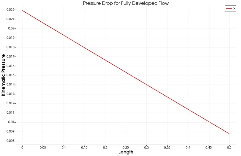Numerical Pressure Drop from above graph=0.022−0.0088=0.0132.

% Dynamic viscosity
mu = 0.89e-3;
% Density 
rho = 997;
%REYNOLDS NUMBER
re=2100;
d=0.0127;
r=d/2;
% Hagen poiseuille flow equations
v_avg = (re*mu)/(rho*d);
v_max = 2*(v_avg);
%Pressure Drop in Fully Developed Flow
del_p = (8*mu*0.5*v_avg)/(r^2)
%Pressure Drop
kinematic_p = del_p/rho
%Kinematic Pressure Drop

Output

del_p =

13.0321

kinematic_p =

0.0131