Week 12 - Symmetry vs Wedge vs HP equation
1. Aim:
To write a program in MATLAB that can generate the computational mesh automatically for any angle and grading schemes and post-process Velocity profile and shear stress. Also, to compare the results obtained using symmetry condition with that of the wedge condition and also the Hagen-Poiseuille's equation.
2. Equations solved:
a. Continuity Equation:
`(delu)/(delx)+(delv)/(dely)+(delw)/(delz)=0`
b. Momentum Equation:
`(delu)/(delt)+u*(nablau)=-(dp)/dx+mu*((del^2u)/(delx^2)+(del^2u)/(dely^2)+(del^2u)/(delz^2))`
`(delv)/(delt)+u*(nablav)=-(dp)/dy+mu*((del^2v)/(delx^2)+(del^2v)/(dely^2)+(del^2v)/(delz^2))`
`(delw)/(delt)+u*(nablaw)=-(dp)/dz+mu*((del^2w)/(delx^2)+(del^2w)/(dely^2)+(del^2w)/(delz^2))`
c. Shear stress equation (solved in post-processing for shear stress plot):
`tau=mu(delu)/(delr)`
3. Simulation Physics and Types of Conditions:
In this case, we are simulating flow through a pipe using OpenFOAM software. The solver used is icoFoam (Incompressible flow). In incompressible flow through a pipe, the density of the moving flow remains constant throughout. The flow condition is set such that the flow is laminar. Because of frictional effects and no-slip condition, the velocity of the fluid becomes zero near the pipe surface. The fluid near the surface of pipe experiences shear force. Due to viscosity of fluid, each layer of fluid exerts a shear force on adjacent layer and the effect of shear force near the surface propagates and the result is the boundary layer phenomenon. And as a result of this boundary layer, the velocity decreases in radial direction as we move along the length of pipe. It keeps decreasing till entrance length is reached. After the entrance length, the flow becomes fully developed. In order to maintain constant mass flow, the flow velocity near the central axis increases in order to accommodate for decreased velocity near surface.
Simulating the flow for the entire geometry of pipe can be time consuming and computationally heavy too. But as the geometry of pipe is symmetrical, we can take a symmetrical section of geometry and perform simulation on it. The two types of conditions are: Wedge and Symmetry. Wedge condition is only accurate for very small angles (less than 5 degree). But for larger angles symmetry condition gives accurate results. These conditions are to be specified in the blockMesh file as well as initial pressure and velocity file.
4. Procedure:
- First of all decide the geometry dimensions (radius of pipe, length of pipe, angle of wedge), flow properties (Temperature, Reynolds number), meshing properties (grading). The length of pipe should be chosen such that it is sufficiently greater than entrance length and so the flow is fully developed. Find out the density, dynamics viscosity and kinematic viscosity at the decided temperature. Also, find out the average flow velocity from Reynolds number equation.
- Write a MATLAB code using file parsing that takes angle of wedge, length of pipe, radius of pipe and grading in x,y,z directions as input and in return generates the blockMesh file for these geometry features. The block should be of the shape of a wedge. The curved surface is defined using 'arc' keyword inside edges part of the code.
- Define the initial pressure and velocity distribution at all boundaries and in internal region at inital time step (t=0) in the p and U file.
- In the transportProperties file, assign the appropriate value of kinematic viscosity to the variable nu.
- In controlDict file, specify time step size and endTime for simulation. Time step size should be such that the Courant number stays less than 1.
- Use blockMesh command in Terminal to generate mesh. Use icoFoam command to run the simulation and use paraFoam to view results in ParaView.
- Plot velocity along radial direction in fully developed region. Export this data and compare it with the wedge case and the Hagen–Poiseuille equation.
- Plot pressure along the length of pipe to find the pressure drop across the length of pipe. Compare it with pressure drop obtained from wedge case and Hagen–Poiseuille equation.
- Finally plot shear stress variation in radial direction by calculating gradient of velocity and multiplying it by dynamic viscosity. Compare it with wedge case and theoretical stress values.
5. Calculations:
For the given problem, we assume the flowing fluid is water and simulation is performed at 25 degree Celsius and flow is laminar. So following are the properties of fluid (water):
Density: `rho=997kg//m^3`
Dynamic Viscosity: `mu=0.0008891Ns//m^2`
Kinematic Viscosity: `nu=mu/rho=0.00000089177m^2//s`
Reynolds number: `Re=2100`
Diameter of Pipe: `D=0.02 m`
Entrance Length: `L_e=0.05*Re*D=2.1m`
Length of Pipe: `L=3m`
Velocity at Entrance: `V_(avg)=(Re*mu)/(rho*D)=0.0936364m//s`
Max Theoretical Velocity: `V_(max)=2*V_(avg)=0.1872728m//s`
Velocity distribution in radial direction according to Hagen-Poiseuille equation: `u=V_(max)(1-r^2/R^2)`
Pressure drop according to Hagen-Poiseuille equation: `DeltaP=(32muLv_(avg))/D^2`
Kinematic pressure drop according to Hagen-Poiseuille equation: `DeltaP_k=(DeltaP)/rho`
6. MATLAB Code for generating blockMesh file:
clc
clear all
close all

theta=45;                            %Angle of Wedge cut out of cylinder (in degrees)
L=3;                                 %Length of pipe (in m)
r=0.01;                              %Radius of Wedge (in m)
g_r=0.1;                             %Grading in radial direction
g_t=1;                               %Grading perpendicular to radial direction
g_a=1;                               %Grading in axial direction

f=fopen('blockMeshDict.txt','w');    %Open file in write mode

fprintf(f,'%s\n','/*--------------------------------*- C++ -*----------------------------------*\');
fprintf(f,'%s\n','| =========                 |                                                 |');
fprintf(f,'%s\n','| \\      /  F ield         | OpenFOAM: The Open Source CFD Toolbox           |');
fprintf(f,'%s\n','|  \\    /   O peration     | Website:  https://openfoam.org                  |');
fprintf(f,'%s\n','|   \\  /    A nd           | Version:  8                                     |');
fprintf(f,'%s\n','|    \\/     M anipulation  |                                                 |');
fprintf(f,'%s\n\n','\*---------------------------------------------------------------------------*/');

fprintf(f,'%s\n','FoamFile');
fprintf(f,'%s\n','{');
fprintf(f,'\t%s\n','version     2.0;');
fprintf(f,'\t%s\n','format      ascii;');
fprintf(f,'\t%s\n','class       dictionary;');
fprintf(f,'\t%s\n','object      blockMeshDict;');
fprintf(f,'%s\n','}');
fprintf(f,'%s\n\n','// * * * * * * * * * * * * * * * * * * * * * * * * * * * * * * * * * * * * * //');

fprintf(f,'%s\n','vertices');
fprintf(f,'%s\n','(');
fprintf(f,'\t(%d %d %d)\n',0,0,0);
fprintf(f,'\t(%d %d %d)\n',r*cosd(theta/2),-r*sind(theta/2),0);
fprintf(f,'\t(%d %d %d)\n',r*cosd(theta/2),r*sind(theta/2),0);
fprintf(f,'\t(%d %d %d)\n',0,0,L);
fprintf(f,'\t(%d %d %d)\n',r*cosd(theta/2),-r*sind(theta/2),L);
fprintf(f,'\t(%d %d %d)\n',r*cosd(theta/2),r*sind(theta/2),L);
fprintf(f,'%s\n\n',');');

fprintf(f,'%s\n','blocks');
fprintf(f,'%s\n','(');
fprintf(f,'\thex (0 1 2 0 3 4 5 3) (50 1 300) simpleGrading (%d %d %d)\n',g_r,g_t,g_a);
fprintf(f,'%s\n\n',');');

fprintf(f,'%s\n','edges');
fprintf(f,'%s\n','(');
fprintf(f,'\tarc 1 2 (%d %d %d)\n',r,0,0);
fprintf(f,'\tarc 4 5 (%d %d %d)\n',r,0,L);
fprintf(f,'%s\n\n',');');

fprintf(f,'%s\n','boundary');
fprintf(f,'%s\n','(');
fprintf(f,'\t%s\n','inlet');
fprintf(f,'\t%s\n','{');
fprintf(f,'\t\t%s\n','type patch;');
fprintf(f,'\t\t%s\n','faces');
fprintf(f,'\t\t%s\n','(');
fprintf(f,'\t\t\t%s\n','(0 2 1 0)');
fprintf(f,'\t\t%s\n',');');
fprintf(f,'\t%s\n','}');
fprintf(f,'\t%s\n','curvedSurface');
fprintf(f,'\t%s\n','{');
fprintf(f,'\t\t%s\n','type wall;');
fprintf(f,'\t\t%s\n','faces');
fprintf(f,'\t\t%s\n','(');
fprintf(f,'\t\t\t%s\n','(1 2 5 4)');
fprintf(f,'\t\t%s\n',');');
fprintf(f,'\t%s\n','}');
fprintf(f,'\t%s\n','front');
fprintf(f,'\t%s\n','{');
fprintf(f,'\t\t%s\n','type symmetry;');
fprintf(f,'\t\t%s\n','faces');
fprintf(f,'\t\t%s\n','(');
fprintf(f,'\t\t\t%s\n','(0 1 4 3)');
fprintf(f,'\t\t%s\n',');');
fprintf(f,'\t%s\n','}');
fprintf(f,'\t%s\n','back');
fprintf(f,'\t%s\n','{');
fprintf(f,'\t\t%s\n','type symmetry;');
fprintf(f,'\t\t%s\n','faces');
fprintf(f,'\t\t%s\n','(');
fprintf(f,'\t\t\t%s\n','(0 3 5 2)');
fprintf(f,'\t\t%s\n',');');
fprintf(f,'\t%s\n','}');
fprintf(f,'\t%s\n','outlet');
fprintf(f,'\t%s\n','{');
fprintf(f,'\t\t%s\n','type patch;');
fprintf(f,'\t\t%s\n','faces');
fprintf(f,'\t\t%s\n','(');
fprintf(f,'\t\t\t%s\n','(3 4 5 3)');
fprintf(f,'\t\t%s\n',');');
fprintf(f,'\t%s\n','}');
fprintf(f,'\t%s\n','axis');
fprintf(f,'\t%s\n','{');
fprintf(f,'\t\t%s\n','type empty;');
fprintf(f,'\t\t%s\n','faces');
fprintf(f,'\t\t%s\n','(');
fprintf(f,'\t\t\t%s\n','(0 3 3 0)');
fprintf(f,'\t\t%s\n',');');
fprintf(f,'\t%s\n','}');
fprintf(f,'%s\n\n',');');

fprintf(f,'%s\n','mergePatchPairs');
fprintf(f,'%s\n','(');
fprintf(f,'%s\n\n',');');

fprintf(f,'%s\n','// ************************************************************************* //');
7. Files for Mesh, Time Control and Initial Conditions:
a. blockMesh File for theta=45:
/*--------------------------------*- C++ -*----------------------------------*\
| =========                 |                                                 |
| \\      /  F ield         | OpenFOAM: The Open Source CFD Toolbox           |
|  \\    /   O peration     | Website:  https://openfoam.org                  |
|   \\  /    A nd           | Version:  8                                     |
|    \\/     M anipulation  |                                                 |
\*---------------------------------------------------------------------------*/

FoamFile
{
	version     2.0;
	format      ascii;
	class       dictionary;
	object      blockMeshDict;
}
// * * * * * * * * * * * * * * * * * * * * * * * * * * * * * * * * * * * * * //

vertices
(
	(0 0 0)
	(0.0092388 -0.00382683 0)
	(0.0092388 0.00382683 0)
	(0 0 3)
	(0.0092388 -0.00382683 3)
	(0.0092388 0.00382683 3)
);

blocks
(
	hex (0 1 2 0 3 4 5 3) (20 5 300) simpleGrading (0.1 1 1)
);

edges
(
	arc 1 2 (0.01 0 0)
	arc 4 5 (0.01 0 3)
);

boundary
(
	inlet
	{
		type patch;
		faces
		(
			(0 2 1 0)
		);
	}
	curvedSurface
	{
		type wall;
		faces
		(
			(1 2 5 4)
		);
	}
	front
	{
		type symmetry;
		faces
		(
			(0 1 4 3)
		);
	}
	back
	{
		type symmetry;
		faces
		(
			(0 3 5 2)
		);
	}
	outlet
	{
		type patch;
		faces
		(
			(3 4 5 3)
		);
	}
	axis
	{
		type empty;
		faces
		(
			(0 3 3 0)
		);
	}
);

mergePatchPairs
(
);

// ************************************************************************* //
b. blockMesh file for theta=25:
/*--------------------------------*- C++ -*----------------------------------*\
| =========                 |                                                 |
| \\      /  F ield         | OpenFOAM: The Open Source CFD Toolbox           |
|  \\    /   O peration     | Website:  https://openfoam.org                  |
|   \\  /    A nd           | Version:  8                                     |
|    \\/     M anipulation  |                                                 |
\*---------------------------------------------------------------------------*/

FoamFile
{
	version     2.0;
	format      ascii;
	class       dictionary;
	object      blockMeshDict;
}
// * * * * * * * * * * * * * * * * * * * * * * * * * * * * * * * * * * * * * //

vertices
(
	(0 0 0)
	(0.00976296 -0.0021644 0)
	(0.00976296 0.0021644 0)
	(0 0 3)
	(0.00976296 -0.0021644 3)
	(0.00976296 0.0021644 3)
);

blocks
(
	hex (0 1 2 0 3 4 5 3) (20 5 300) simpleGrading (0.1 1 1)
);

edges
(
	arc 1 2 (0.01 0 0)
	arc 4 5 (0.01 0 3)
);

boundary
(
	inlet
	{
		type patch;
		faces
		(
			(0 2 1 0)
		);
	}
	curvedSurface
	{
		type wall;
		faces
		(
			(1 2 5 4)
		);
	}
	front
	{
		type symmetry;
		faces
		(
			(0 1 4 3)
		);
	}
	back
	{
		type symmetry;
		faces
		(
			(0 3 5 2)
		);
	}
	outlet
	{
		type patch;
		faces
		(
			(3 4 5 3)
		);
	}
	axis
	{
		type empty;
		faces
		(
			(0 3 3 0)
		);
	}
);

mergePatchPairs
(
);

// ************************************************************************* //
c. blockMesh file for theta=10:
/*--------------------------------*- C++ -*----------------------------------*\
| =========                 |                                                 |
| \\      /  F ield         | OpenFOAM: The Open Source CFD Toolbox           |
|  \\    /   O peration     | Website:  https://openfoam.org                  |
|   \\  /    A nd           | Version:  8                                     |
|    \\/     M anipulation  |                                                 |
\*---------------------------------------------------------------------------*/

FoamFile
{
	version     2.0;
	format      ascii;
	class       dictionary;
	object      blockMeshDict;
}
// * * * * * * * * * * * * * * * * * * * * * * * * * * * * * * * * * * * * * //

vertices
(
	(0 0 0)
	(0.00996195 -0.000871557 0)
	(0.00996195 0.000871557 0)
	(0 0 3)
	(0.00996195 -0.000871557 3)
	(0.00996195 0.000871557 3)
);

blocks
(
	hex (0 1 2 0 3 4 5 3) (15 4 300) simpleGrading (0.05 1 1)
);

edges
(
	arc 1 2 (0.01 0 0)
	arc 4 5 (0.01 0 3)
);

boundary
(
	inlet
	{
		type patch;
		faces
		(
			(0 2 1 0)
		);
	}
	curvedSurface
	{
		type wall;
		faces
		(
			(1 2 5 4)
		);
	}
	front
	{
		type symmetry;
		faces
		(
			(0 1 4 3)
		);
	}
	back
	{
		type symmetry;
		faces
		(
			(0 3 5 2)
		);
	}
	outlet
	{
		type patch;
		faces
		(
			(3 4 5 3)
		);
	}
	axis
	{
		type empty;
		faces
		(
			(0 3 3 0)
		);
	}
);

mergePatchPairs
(
);

// ************************************************************************* //
d. controlDict file:
/*--------------------------------*- C++ -*----------------------------------*\
  =========                 |
  \\      /  F ield         | OpenFOAM: The Open Source CFD Toolbox
   \\    /   O peration     | Website:  https://openfoam.org
    \\  /    A nd           | Version:  8
     \\/     M anipulation  |
\*---------------------------------------------------------------------------*/
FoamFile
{
    version     2.0;
    format      ascii;
    class       dictionary;
    location    "system";
    object      controlDict;
}
// * * * * * * * * * * * * * * * * * * * * * * * * * * * * * * * * * * * * * //

application     icoFoam;

startFrom       startTime;

startTime       0;

stopAt          endTime;

endTime         40.0;

deltaT          0.005;

writeControl    timeStep;

writeInterval   100;

purgeWrite      0;

writeFormat     ascii;

writePrecision  6;

writeCompression off;

timeFormat      general;

timePrecision   6;

runTimeModifiable true;


// ************************************************************************* //
e. U file (Velocity):
/*--------------------------------*- C++ -*----------------------------------*\
  =========                 |
  \\      /  F ield         | OpenFOAM: The Open Source CFD Toolbox
   \\    /   O peration     | Website:  https://openfoam.org
    \\  /    A nd           | Version:  8
     \\/     M anipulation  |
\*---------------------------------------------------------------------------*/
FoamFile
{
    version     2.0;
    format      ascii;
    class       volVectorField;
    object      U;
}
// * * * * * * * * * * * * * * * * * * * * * * * * * * * * * * * * * * * * * //

dimensions      [0 1 -1 0 0 0 0];

internalField   uniform (0 0 0);

boundaryField
{
    inlet
    {
        type            fixedValue;
        value           uniform (0 0 0.0936364);
    }

    curvedSurface
    {
        type            noSlip;
    }

    front
    {
        type            symmetry;
    }

    back
    {
        type            symmetry;
    }

    outlet
    {
    	type		zeroGradient;
    }

    axis
    {
        type            empty;
    }
}

// ************************************************************************* //
f. p file (Pressure):
/*--------------------------------*- C++ -*----------------------------------*\
  =========                 |
  \\      /  F ield         | OpenFOAM: The Open Source CFD Toolbox
   \\    /   O peration     | Website:  https://openfoam.org
    \\  /    A nd           | Version:  8
     \\/     M anipulation  |
\*---------------------------------------------------------------------------*/
FoamFile
{
    version     2.0;
    format      ascii;
    class       volScalarField;
    object      p;
}
// * * * * * * * * * * * * * * * * * * * * * * * * * * * * * * * * * * * * * //

dimensions      [0 2 -2 0 0 0 0];

internalField   uniform 0;

boundaryField
{
    inlet
    {
        type            zeroGradient;
    }

    curvedSurface
    {
        type            zeroGradient;
    }

    front
    {
        type            symmetry;
    }

    back
    {
        type            symmetry;
    }

    outlet
    {
    	type		fixedValue;
    	value		uniform 0;
    }

    axis
    {
        type            empty;
    }
}

// ************************************************************************* //
g. transportProperties file:
/*--------------------------------*- C++ -*----------------------------------*\
  =========                 |
  \\      /  F ield         | OpenFOAM: The Open Source CFD Toolbox
   \\    /   O peration     | Website:  https://openfoam.org
    \\  /    A nd           | Version:  8
     \\/     M anipulation  |
\*---------------------------------------------------------------------------*/
FoamFile
{
    version     2.0;
    format      ascii;
    class       dictionary;
    location    "constant";
    object      transportProperties;
}
// * * * * * * * * * * * * * * * * * * * * * * * * * * * * * * * * * * * * * //

nu              [0 2 -1 0 0 0 0] 0.00000089177;


// ************************************************************************* //
8. Output:
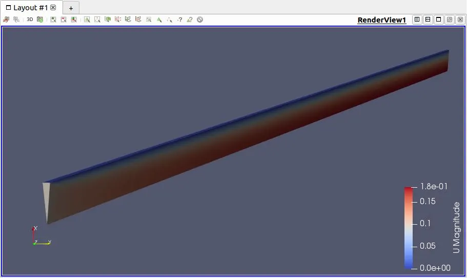
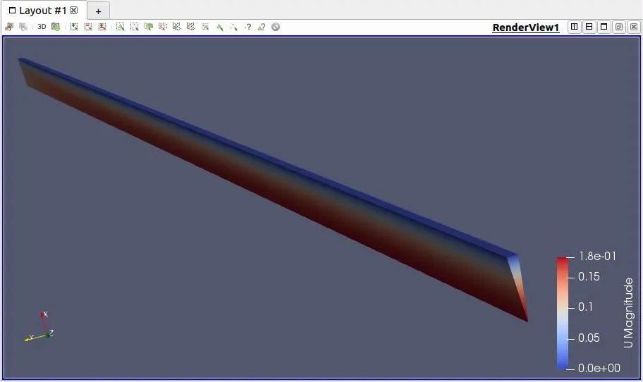
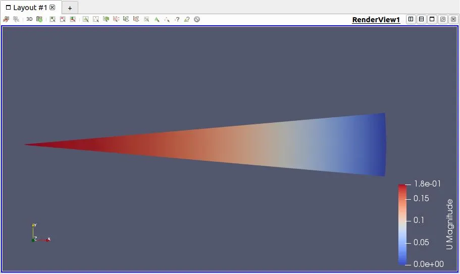
1. Symmetry (theta = 10 deg):
- Velocity contour near the entrance:
- Velocity contour near exit:
- Velocity distribution in radial direction (fully developed region):
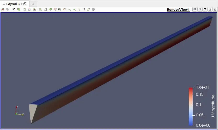
2. Symmetry (theta = 25 deg):
- Velocity contour near the entrance:
- Velocity contour near exit:
- Velocity distribution in radial direction (fully developed region):
3. Symmetry (theta = 45 deg):
- Velocity contour near the entrance:
- Velocity contour near exit:
- Velocity distribution in radial direction (fully developed region):
4. Symmetry vs. Wedge vs. Hagen-Poiseuille equation:
- Comparison of Velocity profile in radial direction in fully developed region (z=2.7m):
- Comparison of Pressure drop in flow direction along axis:
- Shear stress profile in radial direction in fully developed region (z=2.7m):
5. Table of Comparison of Symmetry vs. Wedge vs. Hagen-Poiseuille equation:
| Property | Wedge (2 degree) |
Symmetry (10 degree) |
Symmetry (25 degree) |
Symmetry (45 degree) |
Hagen-Poiseuille Equation |
| Max Velocity (m/s) (z=2.7m) |
0.185879 | 0.182226 | 0.184482 | 0.184499 | 0.1872728 |
| Pressure drop (m2/s2) (from z=2.4m to 3m) |
0.00404837 | 0.00403407 | 0.0040491 | 0.00406579 | 0.004008126 |
| Max Shear stress (N/m2) (z=2.7m) |
0.0330963 | 0.0341289 | 0.0341728 | 0.0342145 | 0.033267548 |
9. Inference and Conclusion:
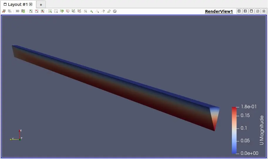
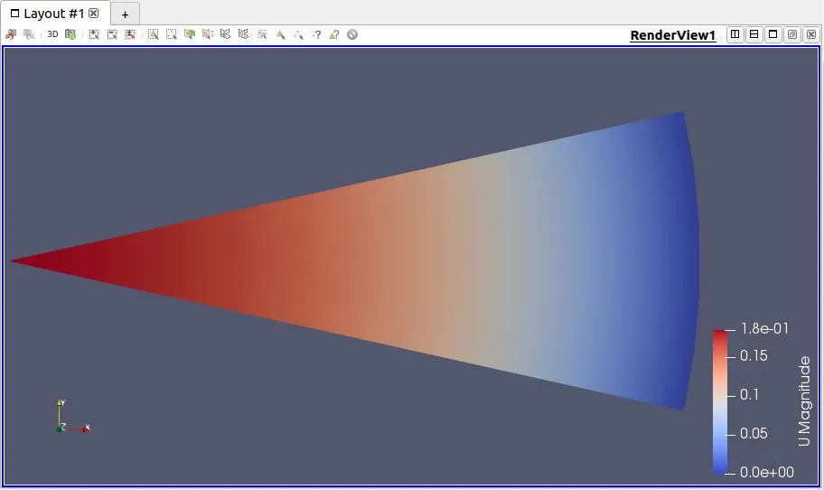
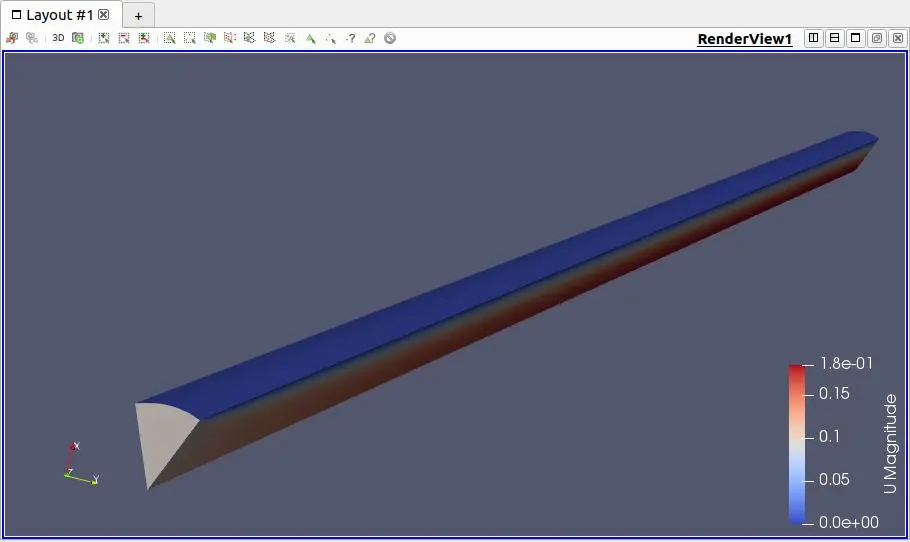
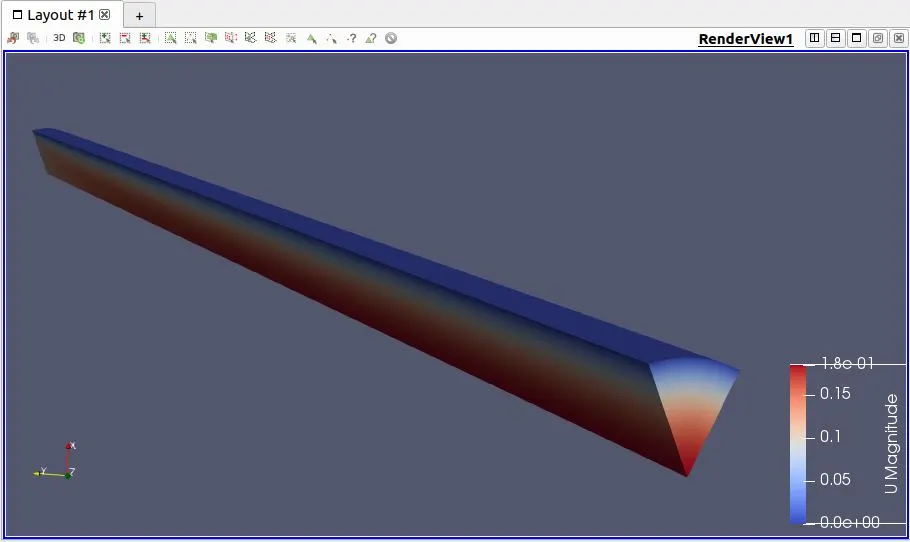
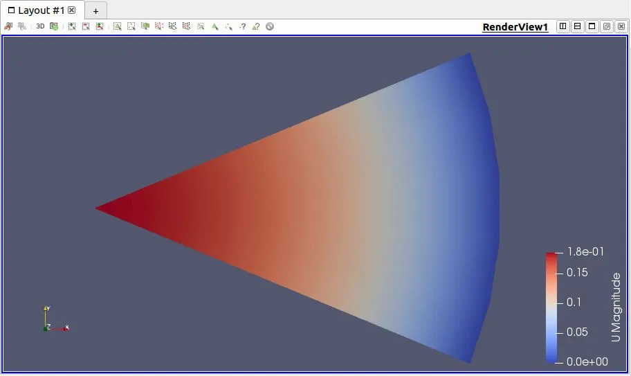
The MATLAB code has successfully generated the desired blockMesh file. The first three parts in output shows velocity contour near the entrance region, exit region and radial distribution in the fully developed region for three different angles of symmetry case. In these contours, we can see that the value of velocity near the entrance is close to 0.1 m/s (0.0936364 precisely). And further ahead in the flow direction, the velocity close to the outer wall starts becoming zero due to no-slip condition. At the exit, we see that velocity near the central axis is close to 0.19 m/s which is almost double that of at the entrance (average velocity). This is expected as `V_(max)=2*V_(avg)`. In this radial distribution contour we can see the effect of boundary layer phenomenon and how it affects the velocity profile in fully developed region. The velocity is maximum near the central axis and drops to zero near the outer surface. The thickness of boundary layer keeps increasing in the flow direction upto the entrance length after which it becomes constant.
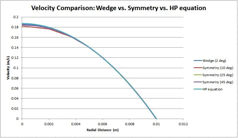
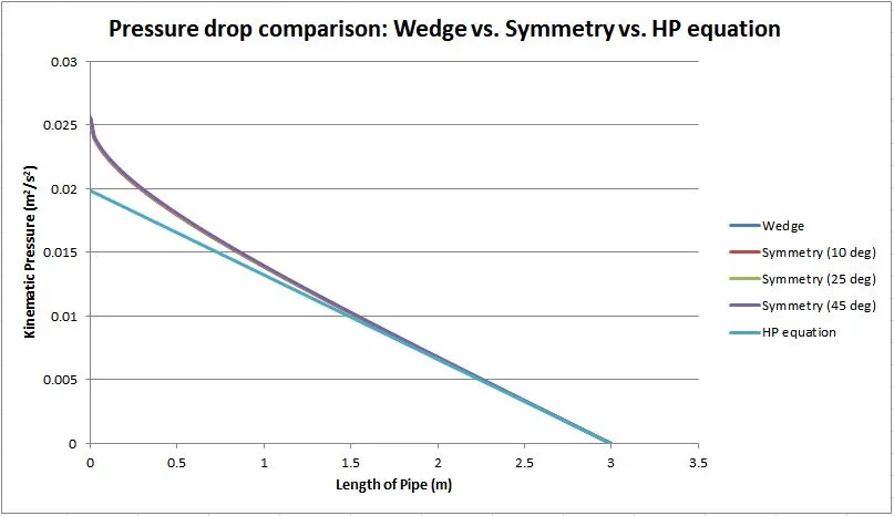
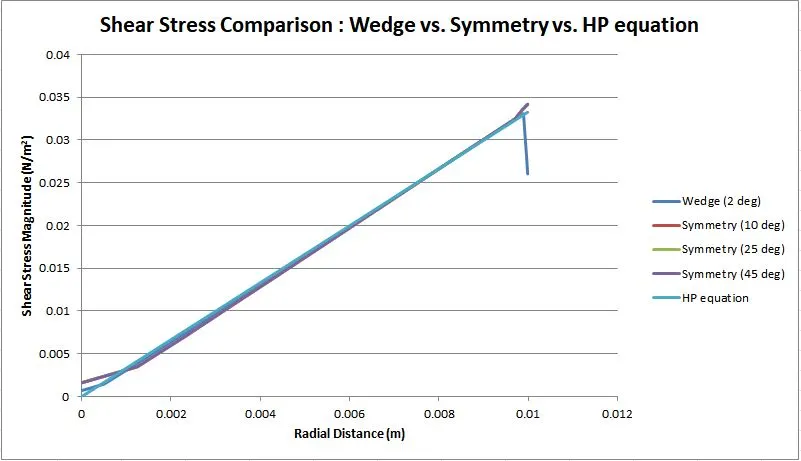
In the fourth part of output, we have compared the wedge case, symmetry case and the Hagen-Poiseuille equation by plotting the velocity distribution in radial direction, pressure drop along the length and shear stress plot. The plot for velocity for all 4 simulated cases overlaps with Hagen-Poiseuille equation. The pressure drop obtained from Hagen-Poiseuille equation holds true in fully developed region. In this case, the entrance length is 2.1m. And so as expected, the pressure drop for all 4 simulated cases overlaps with Hagen-Poiseuille equation after 2.1m. The shear stress plot is directly proportional to gradient of velocity. Since the equation of velocity obtained from Hagen-Poiseuille equation is parabolic in nature, its gradient shoul be linear. And so the shear stress plot for all simulated cases matches with the theoretical stress values (obtained by taking gradient of velocity as per HP equation and multiplying it by dynamic viscosity. There is a small discrepancy in value of shear stress for wedge case in the last cell near the boundary. This may be due to extremely small cell size and taking only single cell in direction perpendicular to radial direction.
In the fifth and final part of output, a comparison table has been made using the data obtained from post-processing. From this, we can see that the values of maximum velocity, pressure drop and maximum shear stress for all four simulated cases is very close to the theoretical values obtained from Hagen-Poiseuille equation and the error is less than of order of 10^-4. Hence, we can say the simulations have been performed correctly. Upon closer observation we see that velocity values are more accurate at larger angles whereas pressure drop and max shear stress values are more accurate for smaller angles. Although the symmetry condition with larger angles is more accurate, it is not always the most feasible method. The symmetry condition with larger angles takes a huge amount of time for computation. So spending so much of time to have slightly more accurate results may not always be the best decision. Instead, we can use the wedge condition with proper meshing and grading schemes. Sometimes on order to capture symmetry angles greater than 5 may be required. In such a case symmetry condition is better as wedge doesn't give accurate results for larger angles. So to conclude, whether to employ the symmetry condition or wedge condition depends on availability of time, computational power and the geometry of the model.