Week 8 - BlockMesh Drill down challenge
1. Aim:
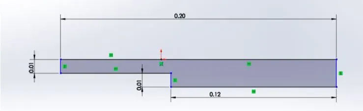
To simulate a 2D flow through a Backward Facing step geometry using OpenFOAM software by producing a block mesh and solving it using icoFOAM solver. And to compare the effects of change in mesh grading on final results.
2. Equations solved:
a. Continuity Equations:
`(delu)/(delx)+(delu)/(dely)=0`
b. Momentum Equation:
`(delu)/(delt)+u*(nablau)=-(delp)/(delx) + mu((del^2u)/(delx^2)+(del^2u)/(dely^2))`
3. Procedure:
The major steps involved in performing this simulation are as follows:
- Deciding which tutorial solves the given problem and the solver it uses: The given simulation involves incompressible flow through a backward facing step. The tutorial for this is inside the incompressible directory of the openFoam tutorials. Open icoFoam inside the incompressible directory. It contains the 'cavity' tutorial which is the one we will solve here.
- Create a copy: Copy this directory and paste it in the openFoam Run directory so that the original files are not changed or corrupted in any way while running the simulation.
- Organisation: Each tutorial contains three main folders - 0, system and constant. 0 folder contains the initial conditions (p and U in this case). system folder contains the mesh generator file, time control file schemes and solution control files.
- Create the geometry: Geometry can be defined by editing the blockMeshDict file in system folder. Define the vertices and using these vertices divide the geometry into blocks. Also define the inlet, outlet, walls and other faces using the faces of these blocks.
- Meshing: Meshing is also defined using blockMeshDict file. Edit the block section of this file to define mesh. For each block define the type of mesh, its vertices, number of cells along each axis and mesh grading factor along each axis.
- Time control: Define the time step size, end time, writing interval and precision by editing the controlDict file.
- Initial Conditions: Define the initial conditions for all applicable variables (p and U here) in internal region and at all defined boundary surfaces like inlet, outlet etc.
- Run the simulation: Run the solver by typing the solver name (icoFoam in this case) in the terminal window when inside the corresponding tutorial directory.
- Open Post-processor: Open paraview post processor using 'paraFoam' command in the terminal window when inside the corresponding tutorial directory.
- Plot Contours: Select the appropriate fields in the properties section and click apply. Now choose the appropriate quantity to plot from the active variable toolbar and the contour will be plotted. Use the time controls to view the contour at any time step.
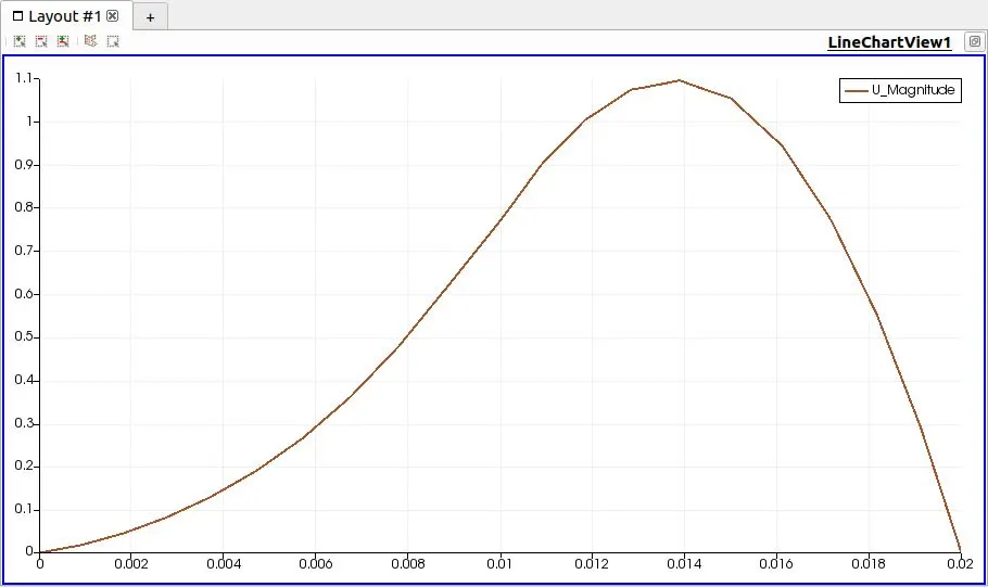
- Velocity line plot: The line plot for velocity at 0.085m from the inlet can be plotted by using the 'plot over line' option in filters menu. Position the two points of line and click apply to plot.
4. Blockmesh Explanation:
- The given geometry can be divided into blocks before meshing it. The blocks and the vertices (in a numbered order) are as shown below:

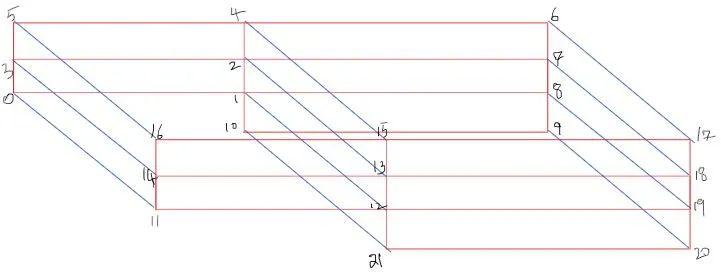
- In the above figure, x-axis is assumed towards the outlet(right), y-axis towards top(up) and z-axis towards front (coming out of plane).
- In the blockMeshDict file, firstly all the vertices are defined. These vertices have an index position starting from 0 in the same order that they are defined. The vertex 0 in the above figure is assumed origin. All the vertices on the back face have z co-ordinate 0. And all the vertices on the front face are 0.1. The inlet is at x=0 and outlet face is at x=0.2. The vertices in the vertical plane of the step have x-coordinate 0.08. The y-coordinate of top surface is 0.01 and bottom surface of step is -0.01. From all this information, all the 22 vertices are defined.
- Using these vertices blocks are defined. The syntax is: hex (0 1 2 3 4 5 6 7) (n1 n2 n3) simpleGrading(g1,g2,g3).
- 'hex' represents that it is a hexahedral mesh. The order of writing the vertices is such that the direction from vertex 0 to 1 represents local x-axis, 1 to 2 represents local y-axis, 2 to 3 represent negative x. Thus the points 0,1,2,3 represent the xy-plane or the back face of block. Similarly the points 4,5,6,7 represent the front face of the blocks. n1,n2,n3 are number of mesh cells in x,y,z directions respectively. g1,g2,g3 is the ratio of the last cell to first cell of that block in x,y,z directions respectively.
- In our case, for grid spacing 0.2, we use either 0.2 or 5 (1/0.2) as grid spacing factor depending on which face of the block the wall lies. For grid spacing 0.5, we use either 0.5 or 2 (1/0.5). For grid spacing 0.8, we use either 0.8 or 1.25 (1/0.8).
- If the wall lies on a face that is in positive x,y,z direction w.r.t. centre of block, then we use 0.2 or 0.5 or 0.8. If the wall lies on a face that is in negative x,y,z direction w.r.t. centre of block, then we use 5 or 2 or 1.25 respectively for each of the three cases.
- Number of cells in x-direction for blocks 1,2 is 80 and blocks 3,4,5 is 120 such that the total cells in x-direction is 200. Number of cells is chosen based on lengths of block in x-direction (0.08 and 0.12). Number of cells in y-direction for 1,2,3,4 blocks is 5 and for fifth block is 10. It is based on lengths of blocks in y-direction (0.05 and 0.1). Number of cells in z-direction is only 1 as it is 2D problem.
- Then we need to define the boundary surfaces (inlet, outlet, fixedWall, frontAndBack). The inlet and outlet are of type 'patch'. fixedWall is of type 'wall'. frontAndBack surfaces are of type 'empty'.
- For defining the boundary surface, we have to mention the faces that make these surfaces. The faces can be defined by using syntax: faces{ (1 2 3 4) (5 6 7 8) ... }.
- The vertices 1,2,3,4 should be mentioned such that when we curl the fingers of right hand in anti-clockwise direction from 1 to 4, the thumb points out of that plane. And if curl the fingers clockwise, the thumb points into the plane.
- After the meshing, we define time step size(dt), endtime and initial conditions and boundary conditions for pressure and velocity.
- The time step (dt) is chosen such that the Courant number (C=U*dt/dx), remains less than 1, where U is the maximum velocity in that cell, and dx or dy is the smallest grid spacing in the entire domain. Here, we have taken dt=0.0001. End time is chosen at 0.1. There are 1000 total time steps. The solution becomes steady after initial few time steps (about 50-60).
5. Code files for Mesh, Time control and initial conditions:
A. blockMeshDict File:
/*--------------------------------*- C++ -*----------------------------------*\
  =========                 |
  \\      /  F ield         | OpenFOAM: The Open Source CFD Toolbox
   \\    /   O peration     | Website:  https://openfoam.org
    \\  /    A nd           | Version:  8
     \\/     M anipulation  |
\*---------------------------------------------------------------------------*/
FoamFile
{
    version     2.0;
    format      ascii;
    class       dictionary;
    object      blockMeshDict;
}
// * * * * * * * * * * * * * * * * * * * * * * * * * * * * * * * * * * * * * //

vertices           // Vertices of the blocks are defined here
(
    (0 0 0)
    (0.08 0 0)
    (0.08 0.005 0)
    (0 0.005 0)
    (0.08 0.01 0)
    (0 0.01 0)
    (0.2 0.01 0)
    (0.2 0.005 0)
    (0.2 0 0)
    (0.2 -0.01 0)
    (0.08 -0.01 0)

    (0 0 0.1)
    (0.08 0 0.1)
    (0.08 0.005 0.1)
    (0 0.005 0.1)
    (0.08 0.01 0.1)
    (0 0.01 0.1)
    (0.2 0.01 0.1)
    (0.2 0.005 0.1)
    (0.2 0 0.1)
    (0.2 -0.01 0.1)
    (0.08 -0.01 0.1)
);

blocks                //Blocks and mesh are defined here
(
    hex (0 1 2 3 11 12 13 14) (80 5 1) simpleGrading (1 5 1)
    hex (3 2 4 5 14 13 15 16) (80 5 1) simpleGrading (1 0.2 1)
    hex (2 7 6 4 13 18 17 15) (120 5 1) simpleGrading (5 0.2 1)
    hex (1 8 7 2 12 19 18 13) (120 5 1) simpleGrading (5 5 1)
    hex (10 9 8 1 21 20 19 12) (120 10 1) simpleGrading (5 5 1)
);

edges
(
);

boundary               //Surface boundaries of the geometry defined here
(
    inlet
    {
        type patch;
        faces
        (
            (0 11 14 3)
            (3 14 16 5)
        );
    }
    fixedWalls
    {
        type wall;
        faces
        (
            (16 15 4 5)
            (15 17 6 4)
            (0 1 12 11)
            (10 9 20 21)
            (10 21 12 1)
        );
    }
    frontAndBack
    {
        type empty;
        faces
        (
            (11 12 13 14)
            (14 13 15 16)
            (13 18 17 15)
            (12 19 18 13)
            (21 20 19 12)
            (1 0 3 2)
            (2 3 5 4)
            (7 2 4 6)
            (8 1 2 7)
            (9 10 1 8)
        );
    }
    outlet
    {
    	type patch;
    	faces
    	(
    	    (18 7 6 17)
    	    (19 8 7 18)
    	    (20 9 8 19)
    	);
    }
);

mergePatchPairs
(
);

// ************************************************************************* //
B. controlDict File:
/*--------------------------------*- C++ -*----------------------------------*\
  =========                 |
  \\      /  F ield         | OpenFOAM: The Open Source CFD Toolbox
   \\    /   O peration     | Website:  https://openfoam.org
    \\  /    A nd           | Version:  8
     \\/     M anipulation  |
\*---------------------------------------------------------------------------*/
FoamFile
{
    version     2.0;
    format      ascii;
    class       dictionary;
    location    "system";
    object      controlDict;
}
// * * * * * * * * * * * * * * * * * * * * * * * * * * * * * * * * * * * * * //

application     icoFoam;

startFrom       startTime;

startTime       0;

stopAt          endTime;

endTime         0.1;

deltaT          0.0001;

writeControl    timeStep;

writeInterval   1;

purgeWrite      0;

writeFormat     ascii;

writePrecision  6;

writeCompression off;

timeFormat      general;

timePrecision   6;

runTimeModifiable true;


// ************************************************************************* //
C. Pressure File (p):
/*--------------------------------*- C++ -*----------------------------------*\
  =========                 |
  \\      /  F ield         | OpenFOAM: The Open Source CFD Toolbox
   \\    /   O peration     | Website:  https://openfoam.org
    \\  /    A nd           | Version:  8
     \\/     M anipulation  |
\*---------------------------------------------------------------------------*/
FoamFile
{
    version     2.0;
    format      ascii;
    class       volScalarField;
    object      p;
}
// * * * * * * * * * * * * * * * * * * * * * * * * * * * * * * * * * * * * * //

dimensions      [0 2 -2 0 0 0 0];

internalField   uniform 0;

boundaryField
{
    inlet
    {
        type            zeroGradient;
    }

    fixedWalls
    {
        type            zeroGradient;
    }

    frontAndBack
    {
        type            empty;
    }

    outlet
    {
    	type		fixedValue;
    	value		uniform 0;
    }
}

// ************************************************************************* //
D. Velocity File (U):
/*--------------------------------*- C++ -*----------------------------------*\
  =========                 |
  \\      /  F ield         | OpenFOAM: The Open Source CFD Toolbox
   \\    /   O peration     | Website:  https://openfoam.org
    \\  /    A nd           | Version:  8
     \\/     M anipulation  |
\*---------------------------------------------------------------------------*/
FoamFile
{
    version     2.0;
    format      ascii;
    class       volVectorField;
    object      U;
}
// * * * * * * * * * * * * * * * * * * * * * * * * * * * * * * * * * * * * * //

dimensions      [0 1 -1 0 0 0 0];

internalField   uniform (0 0 0);

boundaryField
{
    inlet
    {
        type            fixedValue;
        value           uniform (1 0 0);
    }

    fixedWalls
    {
        type            noSlip;
    }

    frontAndBack
    {
        type            empty;
    }

    outlet
    {
    	type		zeroGradient;
    }
}

// ************************************************************************* //
Other files like transportProperties, fvSchemes, fvSolution have been left unchanged.
6. Output:
1. Mesh Grading = 0.2:
- Change in Mesh Code in blockMeshDict File:
blocks //Blocks and mesh are defined here ( hex (0 1 2 3 11 12 13 14) (80 5 1) simpleGrading (1 5 1) hex (3 2 4 5 14 13 15 16) (80 5 1) simpleGrading (1 0.2 1) hex (2 7 6 4 13 18 17 15) (120 5 1) simpleGrading (5 0.2 1) hex (1 8 7 2 12 19 18 13) (120 5 1) simpleGrading (5 5 1) hex (10 9 8 1 21 20 19 12) (120 10 1) simpleGrading (5 5 1) ); - Mesh:
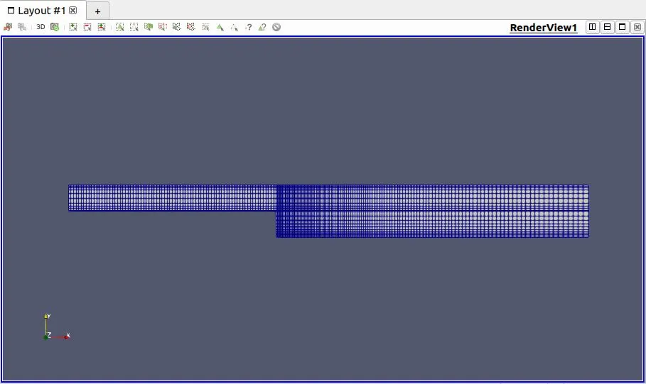
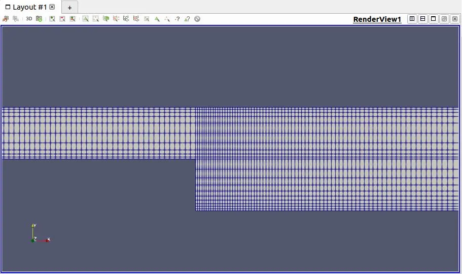
- Closer look at Mesh near the step:
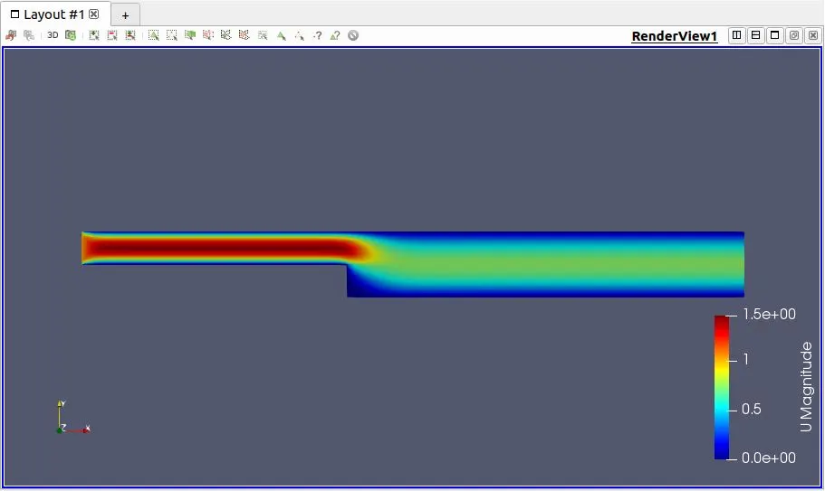
- Velocity Contour:
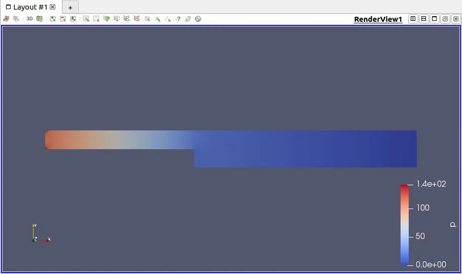
- Pressure Contour:
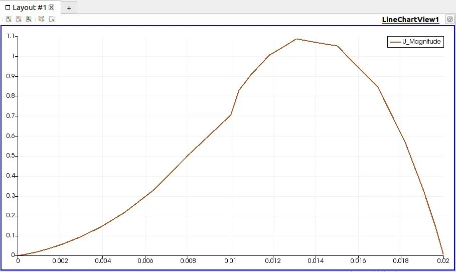
- Velocity Line plot at x=0.085m:
2. Mesh Grading = 0.5:
- Change in Mesh Code in blockMeshDict File:
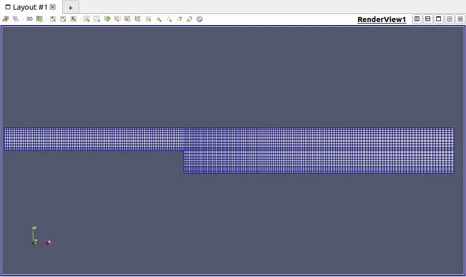
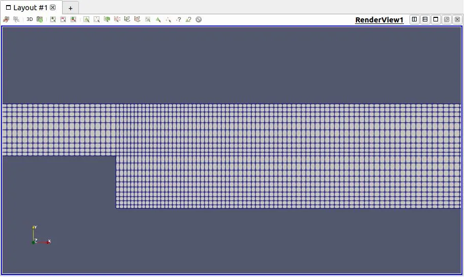
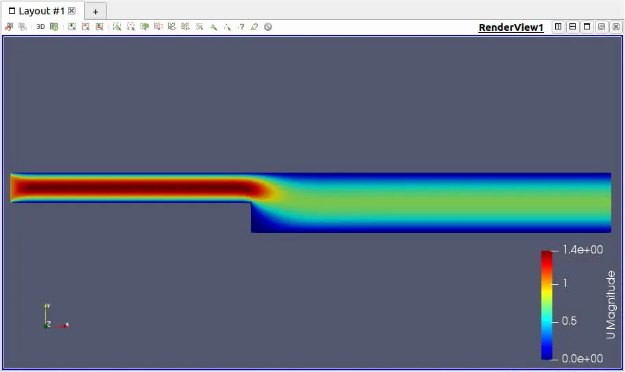
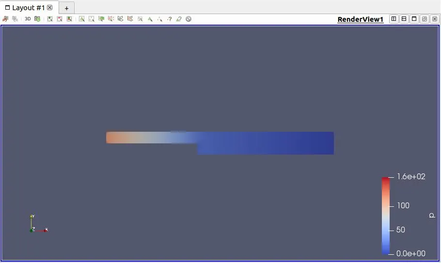
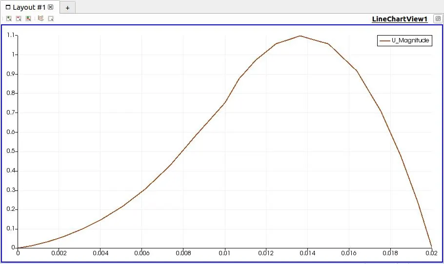
blocks //Blocks and mesh are defined here ( hex (0 1 2 3 11 12 13 14) (80 5 1) simpleGrading (1 2 1) hex (3 2 4 5 14 13 15 16) (80 5 1) simpleGrading (1 0.5 1) hex (2 7 6 4 13 18 17 15) (120 5 1) simpleGrading (2 0.5 1) hex (1 8 7 2 12 19 18 13) (120 5 1) simpleGrading (2 2 1) hex (10 9 8 1 21 20 19 12) (120 10 1) simpleGrading (2 2 1) ); - Mesh:
- Closer look at Mesh near the step:
- Velocity Contour:
- Pressure Contour:
- Velocity Line plot at x=0.085m:
3. Mesh Grading = 0.8:
- Change in Mesh Code in blockMeshDict File:
blocks //Blocks and mesh are defined here ( hex (0 1 2 3 11 12 13 14) (80 5 1) simpleGrading (1 1.25 1) hex (3 2 4 5 14 13 15 16) (80 5 1) simpleGrading (1 0.8 1) hex (2 7 6 4 13 18 17 15) (120 5 1) simpleGrading (1.25 0.8 1) hex (1 8 7 2 12 19 18 13) (120 5 1) simpleGrading (1.25 1.25 1) hex (10 9 8 1 21 20 19 12) (120 10 1) simpleGrading (1.25 1.25 1) ); - Mesh:
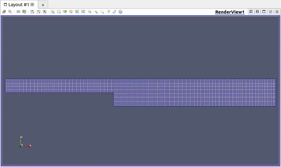
- Closer look at Mesh near the step:
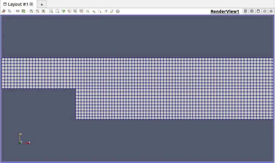
- Velocity Contour:
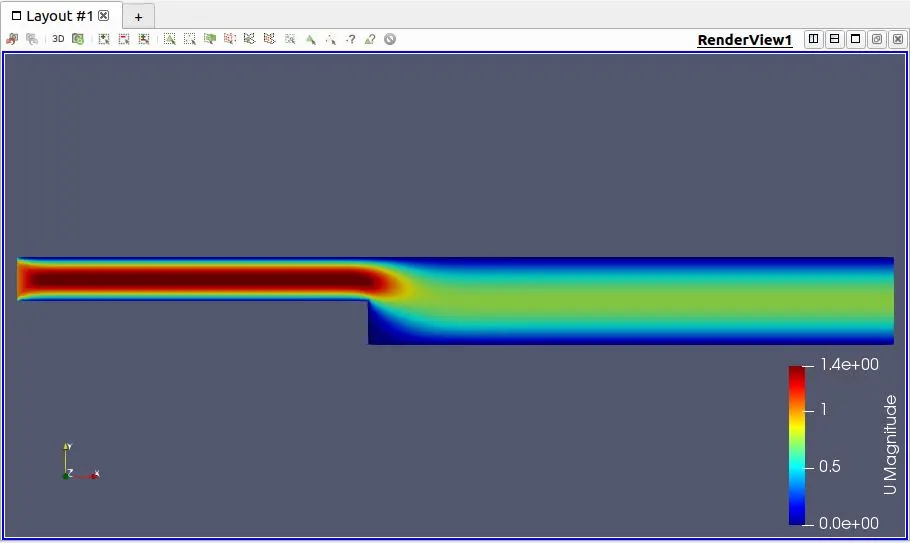
- Pressure Contour:
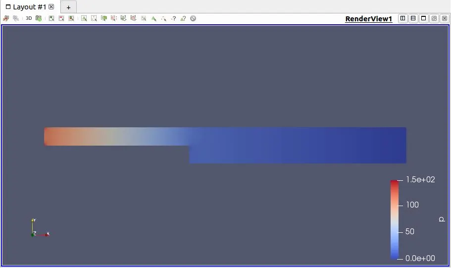
- Velocity Line plot at x=0.085m:
7. Inference and Conclusion:
The velocity and pressure contour are similar for all three mesh grading. The velocity line plot also shows a similar pattern. It slowly increases and reaches a maximum at around 0.014 (0.004 from the central axis or x-axis). And after that begins to drop reaching 0 at the end. The maximum velocity for mesh grading 0.2, 0.5 and 0.8 were found to be 1.087, 1.097 and 1.096 respectively. From the figure and the velocity and pressure data, it seems that grading of 0.2 isn't able to capture maximum velocity as accurately as 0.5 and 0.8. It is obvious because for 0.2, the cells are close together near the wall and wide apart near the centre where velocity is higher. So due to coarse size, it is not as accurate as 0.5 and 0.8. However, grading of 0.8 doesn't capture boundary layer properties as accurately as grading of 0.2 and 0.5 as these grading provide finer mesh size near boundaries. So we can conclude that to accurately calculate both maximum and boundary layer properties, grading of 0.5 is most accurate.