Week 7 - Simulation of a 1D Super-sonic nozzle flow simulation using Macormack Method
1. Aim:
Simulate the isentropic flow through a quasi 1D subsonic-supersonic nozzle for both the conservation and non-conservation forms of the governing equations and solve them using the MacCormack's technique. Determine the steady-state distribution for the flow-field variables and investigate the difference between the two forms of governing equations by comparing their solutions.
2. Theory and Governing Equations:
1. Non-Conservation form:
Continuity equation: `(del(rhoA))/(delt)=-rhoA(delv)/(delx)-rhov(delA)/(delx)-vA(delrho)/(delx)`
Momentum equation: `rho(delv)/(delt)=-rhov(delv)/(delx)-R(rho(delT)/(delx)+T(delrho)/(delx))`
Energy equation: `rhoc_v(delT)/(delt)=-rhovc_v(delT)/(delx)-rhoRT[(delv)/(delx)+v(del(lnA))/(delx)]`
We can non-dimensionalize the primitive variables as follows:
`T'=T/T_0 , rho'=rho/rho_0 , x'=x/L , a_0=sqrt(gammaRT_0) , v'=v/a_0 , t'=t/(L/a_0) , A'=A/(A^star)`
where
`rho',T',v',A',x',t' ->`non-dimensionalized variables
`rho_0, T_0 ->`Reservoir Density and Temperature
`L->` Length of Domain
`a_0->`Speed of sound
`A^star->`Throat area
The non-dimensionalized form of equations is:
Continuity: `(delrho')/(delt')=-rho'(delv')/(delx')-rho'v'(del(lnA'))/(delx')-v'(delrho')/(delx')`
Momentum: `(delv')/(delt')=-v'(delv')/(delx')-1/gamma((delT')/(delx')+(T')/(rho')(delrho')/(delx'))`
Energy: `(delT')/(delt')=-v'(delT')/(delx')-(gamma-1)T'[(delv')/(delx')+v'(del(lnA'))/(delx')]`
Now, we can solve these equations using MacCormack's technique. In this technique, forward differencing is applied to spatial derivatives predict the values of variables. Then this backward differencing is applied on these predicted values to obtain the corrected values. The advantage of using this technique is that it gives accuracy of second order without actually calculating the second order derivative terms in Taylor series, which involve more calculations. The steps in MacCormack's technique are as follows:
- In the predictor step, calculate the predicted time derivative using forward differencing.
- Update the density, temperature and velocity using the predicted time derivative.
- In the corrector step, calculate the corrected time derivative by applying backward differencing on updated values.
- The average time derivative is the mean of predicted and corrected derivative.
- Finally update the values at the beginning of current time step using the average time derivative.
- The inlet and exit conditions are updated by extrapolation.
2. Conservation form:
Continuity equation: `(del(rho'A'))/(delt')=-(del(rho'v'A'))/(delx')`
Momentum equation: `(del(rho'v'A'))/(delt')=-(del(rho'A'v'^2+1/gammap'A'))/(delx')+1/gammap'(delA')/(delx')`
Energy equation: `(del[rho'((e')/(gamma-1)+gamma/2v'^2)A'])/(delt')=-(del[rho'((e')/(gamma-1)+gamma/2v'^2)v'A'+p'v'A'])/(delx')`
If we express the above equations in terms of solutions vector U, flux vector F and Source term J as follows:
`U1=rho'A'`
`U2=rho'v'A'`
`U3=rho'((e')/(gamma-1)+gamma/2v'^2)A'`
`F1=rho'v'A'`
`F2=rho'v'A'+1/gammap'A'`
`F3=rho'((e')/(gamma-1)+gamma/2v'^2)v'A'+p'v'A'`
`J=1/gammap'(delA')/(delx')`
Now the conservation form of equation can be simply written as:
`(delU1)/(delt')=-(delF1)/(delx')`
`(delU2)/(delt')=-(delF2)/(delx')+J`
`(delU3)/(delt')=-(delF3)/(delx')`
Also, the flux terms(F1,F2,F3) can be represented only in terms of solution variables(U1,U2,U3) instead of primitive variables. This is called the pure form of flux terms. It is as follows:
`F1=U2`
`F2=(U_2^2)/U_1+(gamma-1)/gamma(U_3-gamma/2(U_2^2)/U_1)`
`F3=gamma(U_2U_3)/U_1-(gamma(gamma-1))/2(U_2^3)/(U_1^2)`
Now we solve these equations using MacCormack's Technique as follows:
- The initial values of U1,U2,U3 are calculated from initial conditions.
- F1,F2,F3 are calculated from U1,U2,U3 using above pure form equations.
- In the predictor step, calculate the predicted time derivative of U1,U2,U3 using forward differencing of F1,F2,F3.
- Update U1,U2,U3 using the predicted time derivative and from these values of U1,U2,U3 calculate F1,F2,F3.
- In the corrector step, calculate the corrected time derivative of U1,U2,U3 by applying backward differencing on updated values F1,F2,F3.
- The average time derivative is the mean of predicted and corrected derivative.
- Finally update the values of U1,U2,U3 at the beginning of current time step using the average time derivative.
- The inlet and exit conditions are updated by extrapolation.
For plotting, the primitive values (density, velocity, temperature) can be found from U1,U2,U3 as follows:
`rho'=(U1)/(A')`
`v'=(U2)/(U1)`
`T'=(gamma-1)((U3)/(U1)-gamma/2v'^2)`
`p'=rho'T'`
3. MATLAB Code:
Main Code:
clear all
close all
clc

L=3;                                 %Length of nozzle
n=31;                                %Grid points
x=linspace(0,L,n);                   %Locations of grid points
dx=L/(n-1);                          %Grid spacing

m_cons=conservative(x,dx,n);         %Calling conservative function
m_noncons=nonconservative(x,dx,n);   %Calling nonconservative function

figure();
plot(x,m_cons,x,m_noncons);          %Plotting mass flow rate at steady state for conservative and nonconservative
xlabel('Nozzle Length'), ylabel('Non-Dimensionalized Mass flow rate');
title('Comparison of Mass flow rate for Conservative and Non-Conservative equations');
legend('Conservative','Non-Conservative');
Function Code for solving conservation form of equation:
function m_ss = conservative(x,dx,n)
  global z=1;                           %Control variable for mass flow rate plots at different time steps
  gamma=1.4;
  nt=1400;                              %Number of time steps
  dt=0.0267;                            %Time step size
  A=1+2.2*(x-1.5).^2;                   %Area in terms of x

  for i=1:length(x)                     %Density and Temperature initialization
    if x(i)<=0.5
      rho(i)=1.0;
      T(i)=1.0;
    elseif x(i)<=1.5
      rho(i)=1-0.366*(x(i)-0.5);
      T(i)=1.0-0.167*(x(i)-0.5);
    elseif x(i)<=3.0
      rho(i)=0.634-0.3879*(x(i)-1.5);
      T(i)=0.833-0.3507*(x(i)-1.5);
    endif
  endfor

  v=(0.59)./(rho.*A);                   %Velocity initialization
  U1=rho.*A;                            %U1 initialization
  U2=rho.*v.*A;                         %U2 initialization
  U3=U1.*(T/(gamma-1)+(gamma*v.^2)/2);  %U3 initialization

  for k=1:nt
    %Creating a copy of initial U1,U2,U3
    U1_old=U1;
    U2_old=U2;
    U3_old=U3;

    term1=(gamma/2)*(U2.^2)./U1;
    term2=(gamma-1)/gamma;

    %Computing F1,F2,F3 from U1,U2,U3
    F1=U2;
    F2=((U2.^2)./U1)+term2*(U3-term1);
    F3=U2./U1.*(gamma*U3-term1*(gamma-1));

    %Predictor Step
    for i=2:n-1

      %Calculating J2 term
      J2=(1/gamma)*rho(i)*T(i)*((A(i+1)-A(i))/dx);

      dU1dt_pred(i)=-(F1(i+1)-F1(i))/dx;
      dU2dt_pred(i)=-(F2(i+1)-F2(i))/dx + J2;
      dU3dt_pred(i)=-(F3(i+1)-F3(i))/dx;

      %Updating U1,U2,U3 values
      U1(i)=U1(i)+dU1dt_pred(i)*dt;
      U2(i)=U2(i)+dU2dt_pred(i)*dt;
      U3(i)=U3(i)+dU3dt_pred(i)*dt;
    endfor

    %Updating U2 and U3 at inlet (U1 is constant at inlet because rho at inlet is assumed constant)
    U2(1)=2*U2(2)-U2(3);
    U3(1)=U1(1)*(T(1)/(gamma-1)+(gamma*v(1)^2)/2);

    term1=(gamma/2)*(U2.^2)./U1;
    term2=(gamma-1)/gamma;

    %Computing F1,F2,F3 from U1,U2,U3
    F1=U2;
    F2=((U2.^2)./U1)+term2*(U3-term1);
    F3=U2./U1.*(gamma*U3-term1*(gamma-1));

    %Updating rho and T to calculate J2
    rho=U1./A;
    v=U2./U1;
    T=(gamma-1)*(U3./U1-gamma/2*(v.^2));

    %Corrector Step
    for i=2:n-1

      %Calculating J2 term
      J2=(1/gamma)*rho(i)*T(i)*((A(i)-A(i-1))/dx);

      dU1dt_corr(i)=-(F1(i)-F1(i-1))/dx;
      dU2dt_corr(i)=-(F2(i)-F2(i-1))/dx + J2;
      dU3dt_corr(i)=-(F3(i)-F3(i-1))/dx;
    endfor

    %Calculating time derivative of U1,U2,U3
    dU1dt=0.5*(dU1dt_pred+dU1dt_corr);
    dU2dt=0.5*(dU2dt_pred+dU2dt_corr);
    dU3dt=0.5*(dU3dt_pred+dU3dt_corr);

    %Updating U1,U2,U3 values
    for i=2:n-1
      U1(i)=U1_old(i)+dU1dt(i)*dt;
      U2(i)=U2_old(i)+dU2dt(i)*dt;
      U3(i)=U3_old(i)+dU3dt(i)*dt;
    endfor

    %Updating U1,U2,U3 at exit
    U1(n)=2*U1(n-1)-U1(n-2);
    U2(n)=2*U2(n-1)-U2(n-2);
    U3(n)=2*U3(n-1)-U3(n-2);

    %Calculating primitive variables from U1,U2,U3
    rho=U1./A;                             %Density
    v=U2./U1;                              %Velocity
    T=(gamma-1)*(U3./U1-gamma/2*(v.^2));   %Temperature
    p=rho.*T;                              %Pressure

##    %Plotting and creating a GIF to show time-wise variation of primitive variables
##    figure();
##    subplot(2,2,1);
##    plot(x,rho);
##    axis([0 3 -0.2 1.5]);
##    xlabel('Nozzle Length'), ylabel('Non-Dimensionalized Density');
##    title(sprintf('Time variation of Density, Time Step: %d',k));
##    subplot(2,2,2);
##    plot(x,v);
##    axis([0 3 -0.2 2.2]);
##    xlabel('Nozzle Length'), ylabel('Non-Dimensionalized Velocity');
##    title(sprintf('Time variation of Velocity, Time Step: %d',k));
##    subplot(2,2,3);
##    plot(x,T);
##    axis([0 3 -0.2 1.5]);
##    xlabel('Nozzle Length'), ylabel('Non-Dimensionalized Temperature');
##    title(sprintf('Time variation of Temperature, Time Step: %d',k));
##    subplot(2,2,4);
##    plot(x,p);
##    axis([0 3 -0.2 1.5]);
##    xlabel('Nozzle Length'), ylabel('Non-Dimensionalized Pressure');
##    title(sprintf('Time variation of Pressure, Time Step: %d',k));
##
##    img = print('-RGBImage');
##    imwrite(img,'animation1.gif','DelayTime',.005,'Compression','bzip','WriteMode','Append');

    %Storing mass flow rate value at intermediate time steps
    if (k==50 || k==100 || k==200 || k==300 || k==500 || k==700 || k==1400)
      global z;
      m(z,:)=rho.*v.*A;
      z=z+1;
    endif
  endfor

  %Plotting mass flow rate at intermediate time steps
  figure();
  for i=1:z-1
    plot(x,m(i,:));
    hold on;
  endfor
  xlabel('Nozzle Length'), ylabel('Non-Dimensionalized Mass Flow rate');
  title('Mass flow rate after different time steps');
  legend('50 time steps','100 time steps','200 time steps','300 time steps','500 time steps','700 time steps','1400 time steps');

  %Plotting Steady-State Distribution of Primitive Variables
  figure();
  subplot(2,2,1);
  plot(x,rho);
  axis([0 3 -0.2 1.2]);
  xlabel('Nozzle Length'), ylabel('Non-Dimensionalized Density');
  title('Steady State Distribution of Density');
  subplot(2,2,2);
  plot(x,v);
  axis([0 3 -0.2 2.2]);
  xlabel('Nozzle Length'), ylabel('Non-Dimensionalized Velocity');
  title('Steady State Distribution of Velocity');
  subplot(2,2,3);
  plot(x,T);
  axis([0 3 -0.2 1.2]);
  xlabel('Nozzle Length'), ylabel('Non-Dimensionalized Temperature');
  title('Steady State Distribution of Temperature');
  subplot(2,2,4);
  plot(x,p);
  axis([0 3 -0.2 1.2]);
  xlabel('Nozzle Length'), ylabel('Non-Dimensionalized Pressure');
  title('Steady State Distribution of Pressure');

  m_ss=m(end,:);              %Returning the steady state mass flow rate
endfunction
Function Code for solving non-conservation form of equation:
function m_ss = nonconservative(x,dx,n)
  global z=1;                           %Control variable for mass flow rate plots at different time steps
  gamma=1.4;
  nt=1400;                              %Number of time steps
  dt=0.0267;                            %Time step size

  rho=1-0.3146*x;                       %Density initialization
  T=1-0.2314*x;                         %Temperature initialization
  v=(0.1+1.09*x).*T.^0.5;               %Velocity initialization
  A=1+2.2*(x-1.5).^2;                   %Area in terms of x

  for k=1:nt
    %Creating a copy of initial conditions
    rho_old=rho;
    v_old=v;
    T_old=T;

    %Predictor step
    for j=2:n-1
      drhodx=(rho(j+1)-rho(j))/dx;
      dvdx=(v(j+1)-v(j))/dx;
      dTdx=(T(j+1)-T(j))/dx;
      dlogAdx=(log(A(j+1))-log(A(j)))/dx;

      drhodt_pred(j)=-rho(j)*dvdx - rho(j)*v(j)*dlogAdx - v(j)*drhodx;     %Continuity equation
      dvdt_pred(j)=-v(j)*dvdx - 1/(gamma)*(dTdx + (T(j)/rho(j))*drhodx);   %Momentum equation
      dTdt_pred(j)=-v(j)*dTdx - (gamma-1)*T(j)*(dvdx + v(j)*dlogAdx);      %Energy equation

      %Updating values
      rho(j)=rho(j)+drhodt_pred(j)*dt;
      v(j)=v(j)+dvdt_pred(j)*dt;
      T(j)=T(j)+dTdt_pred(j)*dt;
    endfor

    %Corrector step
    for j=2:n-1
      drhodx=(rho(j)-rho(j-1))/dx;
      dvdx=(v(j)-v(j-1))/dx;
      dTdx=(T(j)-T(j-1))/dx;
      dlogAdx=(log(A(j))-log(A(j-1)))/dx;

      drhodt_corr(j)=-rho(j)*dvdx - rho(j)*v(j)*dlogAdx - v(j)*drhodx;     %Continuity equation
      dvdt_corr(j)=-v(j)*dvdx - 1/(gamma)*(dTdx + (T(j)/rho(j))*drhodx);   %Momentum equation
      dTdt_corr(j)=-v(j)*dTdx - (gamma-1)*T(j)*(dvdx + v(j)*dlogAdx);      %Energy equation
    endfor

    %Calculating time derivative of density, velocity and temperature
    drhodt=0.5*(drhodt_pred+drhodt_corr);
    dvdt=0.5*(dvdt_pred+dvdt_corr);
    dTdt=0.5*(dTdt_pred+dTdt_corr);

    %Updating final values
    for j=2:n-1
      rho(j)=rho_old(j)+drhodt(j)*dt;
      v(j)=v_old(j)+dvdt(j)*dt;
      T(j)=T_old(j)+dTdt(j)*dt;
    endfor

    %Updating inlet conditions (Temperature and Density assumed constant at inlet)
    v(1)=2*v(2)-v(3);

    %Updating exit conditions
    rho(n)=2*rho(n-1)-rho(n-2);
    v(n)=2*v(n-1)-v(n-2);
    T(n)=2*T(n-1)-T(n-2);

    %Calculating pressure
    p=rho.*T;

##    %Plotting and creating a GIF to show time-wise variation of primitive variables
##    figure(1);
##    subplot(2,2,1);
##    plot(x,rho);
##    axis([0 3 -0.2 1.5]);
##    xlabel('Nozzle Length'), ylabel('Non-Dimensionalized Density');
##    title(sprintf('Time variation of Density, Time Step: %d',k));
##    subplot(2,2,2);
##    plot(x,v);
##    axis([0 3 -0.2 2.2]);
##    xlabel('Nozzle Length'), ylabel('Non-Dimensionalized Velocity');
##    title(sprintf('Time variation of Velocity, Time Step: %d',k));
##    subplot(2,2,3);
##    plot(x,T);
##    axis([0 3 -0.2 1.5]);
##    xlabel('Nozzle Length'), ylabel('Non-Dimensionalized Temperature');
##    title(sprintf('Time variation of Temperature, Time Step: %d',k));
##    subplot(2,2,4);
##    plot(x,p);
##    axis([0 3 -0.2 1.5]);
##    xlabel('Nozzle Length'), ylabel('Non-Dimensionalized Pressure');
##    title(sprintf('Time variation of Pressure, Time Step: %d',k));
##
##    img = print('-RGBImage');
##    imwrite(img,'animation2.gif','DelayTime',.005,'Compression','bzip','WriteMode','Append');

    %Storing mass flow rate value at intermediate time steps
    if (k==50 || k==100 || k==200 || k==300 || k==500 || k==700 || k==1400)
      global z;
      m(z,:)=rho.*v.*A;
      z=z+1;
    endif
  endfor

  %Plotting mass flow rate at intermediate time steps
  figure();
  for i=1:z-1
    plot(x,m(i,:));
    hold on;
  endfor
  xlabel('Nozzle Length'), ylabel('Non-Dimensionalized Mass Flow rate');
  title('Mass flow rate after different time steps');
  legend('50 time steps','100 time steps','200 time steps','300 time steps','500 time steps','700 time steps','1400 time steps');

  %Plotting Steady-State Distribution of Primitive Variables
  figure();
  subplot(2,2,1);
  plot(x,rho);
  axis([0 3 -0.2 1.2]);
  xlabel('Nozzle Length'), ylabel('Non-Dimensionalized Density');
  title('Steady State Distribution of Density');
  subplot(2,2,2);
  plot(x,v);
  axis([0 3 -0.2 2.2]);
  xlabel('Nozzle Length'), ylabel('Non-Dimensionalized Velocity');
  title('Steady State Distribution of Velocity');
  subplot(2,2,3);
  plot(x,T);
  axis([0 3 -0.2 1.2]);
  xlabel('Nozzle Length'), ylabel('Non-Dimensionalized Temperature');
  title('Steady State Distribution of Temperature');
  subplot(2,2,4);
  plot(x,p);
  axis([0 3 -0.2 1.2]);
  xlabel('Nozzle Length'), ylabel('Non-Dimensionalized Pressure');
  title('Steady State Distribution of Pressure');

  m_ss=m(end,:);              %Returning the steady state mass flow rate
endfunction
4. Outputs:
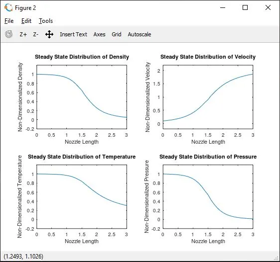
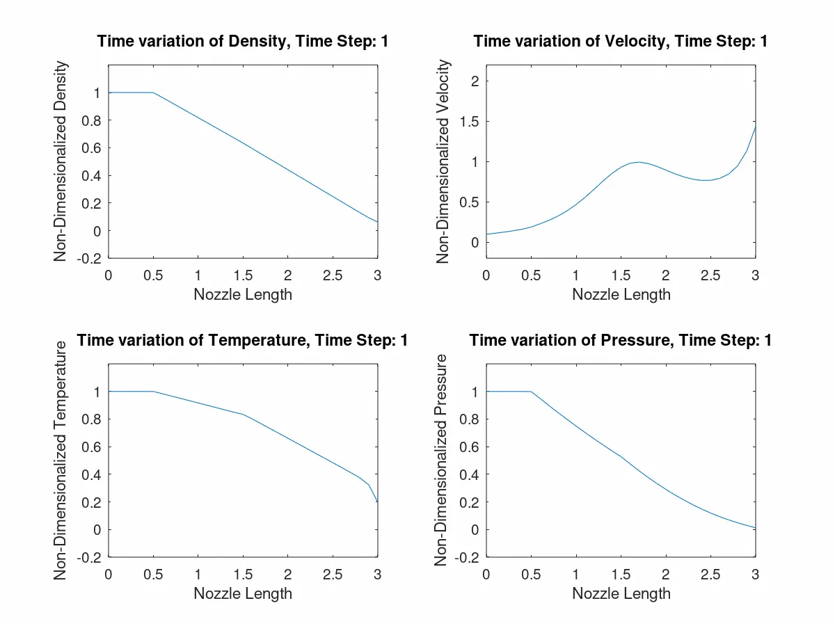
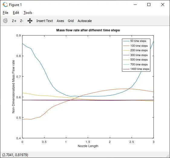
1. Conservation Form of Equation: (31 grid points)
- Steady-state distribution of primitive variables inside the nozzle:
- Time-wise variation of the primitive variables (GIF Animation)(only till 260 time steps because of large file size):
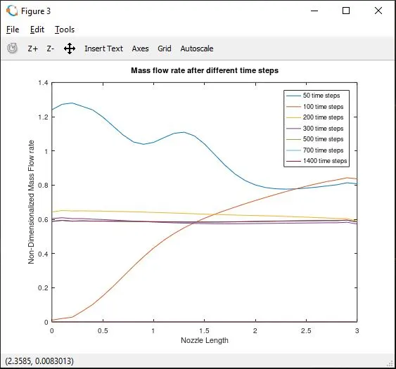
- Variation of Mass flow rate distribution inside the nozzle at different time steps during the time-marching process:
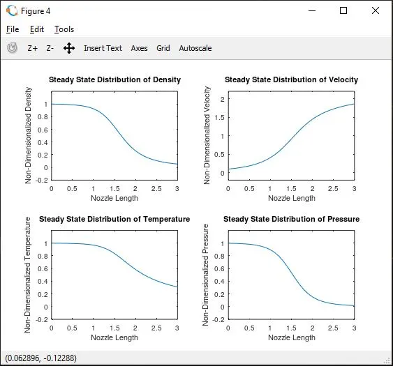
2. Non-Conservation Form of Equation: (31 grid points)
- Steady-state distribution of primitive variables inside the nozzle:
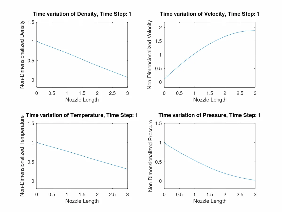
- Time-wise variation of the primitive variables (GIF Animation)(only till 290 time steps because of large file size):
- Variation of Mass flow rate distribution inside the nozzle at different time steps during the time-marching process:
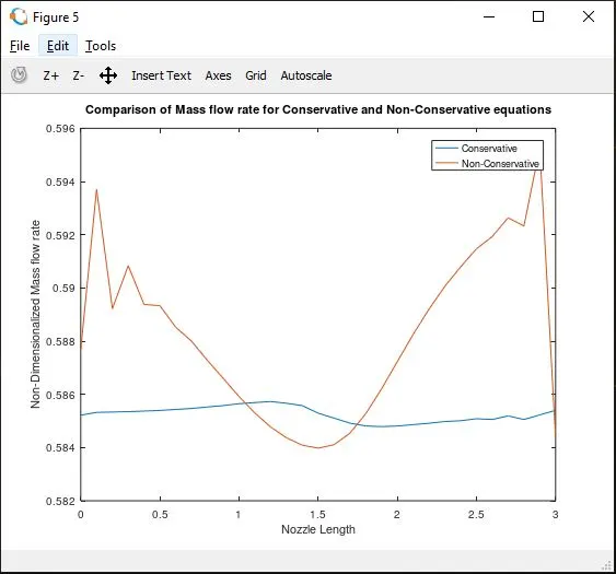
3. Comparison of Normalized mass flow rate distributions of both forms:
5. Inference and Conclusion:
In the plots section we have seen for both conservation and non-conservation equations: the steady state distribution of primitive variables, time-wise variation of primitive variables using a GIF file and variation of Mass flow rate distribution at different time steps. And at the end, we have also compared the mass flow rate distribution at steady state for conservation vs non-conservation.
From the plots, we can see that steady state distribution for primitive variables is same for both equations. Although the distribution at intermediate time steps is different for both equations, they both reach steady state eventually. Also, the mass flow rate distribution becomes steady and similar for both case after about 500-600 time steps. Conservative approach seems better in this case as the steady-state mass flow rate distribution for non-conservative is slightly abrupt near the inlet and exit boundaries.
The steady state values of density, velocity, temperature and pressure were compared at throat section for different number of grid points for both methods. The results are as follows:
| Grid Points | Density | Velocity | Temperature | Pressure | |
| Exact analytical solution | -- | 0.634 | 0.913 | 0.833 | 0.528 |
| Conservation | 31 | 0.64821 | 0.90293 | 0.83891 | 0.54379 |
| 61 | 0.63906 | 0.91206 | 0.83575 | 0.53410 | |
| Non-Conservation | 31 | 0.63898 | 0.91391 | 0.83657 | 0.53456 |
| 61 | 0.63769 | 0.91386 | 0.83546 | 0.53276 |
From the above data, we see that the values for grid points 31 and 61 are very close. And so we can safely take 31 grid points for our calculations without affecting the results. Another thing that we see is that although the mass flow rate for conservation equation was much smoother than non-conservation equation, the values for primitive variables obtained through non-conservation are closer to the actual analytical solution. And hence, non-conservation gives more accurate results in this case.