Simulation of Flow through a pipe in OpenFoam
AIM:
The aim of this project is to simulate the fully developed Hagen poiseuille's flow through a circular pipe. (Re = 2100)
PROCEDURE:
The simulation of flow through a pipe would require huge computational power so we simulate a portion of it. A wedge which is a small part of the circular pipe will be simulated in this project.
The assumptions that come with the Hagen poiseuille’s flow are
-
The flow is incompressible, laminar, Newtonian, and is flowing through a long cylindrical pipe of constant crosssection. There is no acceleration of fluid in the pipe
-
For a fully developed flow, the length of the pipe must be very much greater than the diameter of the pipe.
-
The diameter of the pipe is 0.01 m Therefore we can calculate the hydrodynamic entrance length of the pipe using
Referenced from FM white Le = 0.06 x Re x D. Where D is the diameter of the pipe.
Le = 0.06 x 2100 x 0.01
Le = 1.26m
The hydrodynamic entrance length is the length of the pipe through which a fluid travels before becoming a fully developed flow. The flow would have the velocity profile as shown.
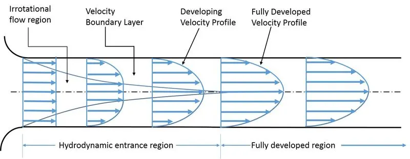
The above picture is taken from a Wikipedia article.
We assume that the pipe length is greater than hydrodynamic entrance length. Lpipe = 1.5 m
And since the fluid inside the pipe is water we take the properties of water at NTP
`20^{o}`C and 1atm
Density `rho = 998 {kg}/m^3`
Dynamic Viscosity `mu = 0.00089 {Ns} / m^2`
Kinematic Viscosity `nu = 1.005e-6 m^2/ s`
`V_{avg} = { Re . mu } /{rho . D }`= 0.187 m/s
`V_max = 2 .V_(avg)`= 0.374 m/s
`Delta P = { 8 .mu . L .V_(avg) } / r^2`= 79.88 pa
`Delta P_k = {Delta P} / { rho }`= 0.080 (m/s)^2
`tau = mu . {dx} /{ dy}`
We use the post-processing software i.e ., ParaView to plot shear stress graph
To input our geometry into OpenFOAM we need to edit the blockMeshDict file. We need to input the vertices for the following orientation.
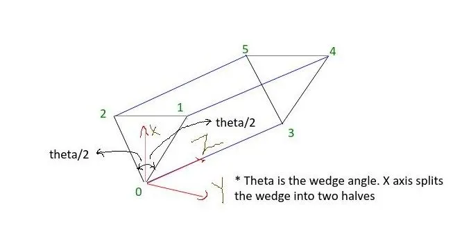
For various wedge angles 2,3,4 deg we need to input these vertices into the blockMestDict file. This method can be automated by using MatLab. We use the following method. We first calculate the vertices using trigonometric formulae.
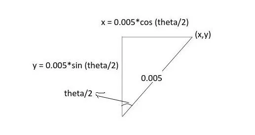
So the formulae for finding the coordinates are as shown. For different wedge angles just with the change in coordinates, we can change the vertices by automating this process.
A block needs 8 vertices in order. But since we have only 6 we repeat the starting vertices at the end. We enter the arc 12 and 45 in the edges tab. Also, we give the number of grids based on the block size and size of the grid.
For automation, the Matlab code is as shown.
clear
close all
clc

%This program is to automate the process of Generating the blockMeshDict
%file which holds the geometrical data in OpenFOAM.

%inputs
%reynolds number
Re = 2100;

%All quantities are taken in SI units

%Diameter of the pipe assumed
Dpipe = 0.01;

%radius
Radpipe = Dpipe/2;

%calculating the hydrodynamic entrance length
Le = 0.06*Re*Dpipe;

%length of the pipe based on the hydrodynamic entrance length (Lpipe > Le)
Lpipe = 1.5;

str = 'What is the wegde angle?';
str = [str newline ''];

%Wedge angle
answer = questdlg(str,'Question','2','3','4','2');
w_a = str2double(answer);

%finding the coordinates of
corx1 = Radpipe*cosd(w_a/2);

cory1 = Radpipe*sind(w_a/2);

corx2 = Radpipe*cosd(-w_a/2);

cory2 = Radpipe*sind(-w_a/2);


f1 = fopen('blockMeshDict','wt');

fprintf(f1,"/*--------------------------------*- C++ -*----------------------------------*      n");
fprintf(f1,"  =========                |n");
fprintf(f1,"        /  F ield         | OpenFOAM: The Open Source CFD Toolboxn");
fprintf(f1,"       /   O peration     | Website:  https://openfoam.orgn");
fprintf(f1,"      /    A nd           | Version:  8n");
fprintf(f1,"     /     M anipulation  |n");
fprintf(f1,"/*---------------------------------------------------------------------------*/n");
fprintf(f1,"FoamFilen");
fprintf(f1,"{n");
fprintf(f1,"    version     2.0;n");
fprintf(f1,"    format      ascii;n");
fprintf(f1,"    class       dictionary;n");
fprintf(f1,"    object      blockMeshDict;n");
fprintf(f1,"}n");
fprintf(f1,"// * * * * * * * * * * * * * * * * * * * * * * * * * * * * * * * * * * * * * //n");
fprintf(f1,"n");
fprintf(f1,"convertToMeters 1;n");
fprintf(f1,"n");
fprintf(f1,"verticesn");
fprintf(f1,"(n");
fprintf(f1,"t(0 0 0)//0n");
fprintf(f1,"t(%f %f 0)//1n",corx1,cory1);
fprintf(f1,"t(%f %f 0)//2n",corx2,cory2);
fprintf(f1,"t(0 0 %f)//3n",Lpipe);
fprintf(f1,"t(%f %f %f)//4n",corx1,cory1,Lpipe);
fprintf(f1,"t(%f %f %f)//5n",corx2,cory2,Lpipe);
fprintf(f1,");n");
fprintf(f1,"n");
fprintf(f1,"n");
fprintf(f1,"blocksn");
fprintf(f1,"(n");
fprintf(f1,"t hex (0 2 1 0 3 5 4 3) (10 1 3000)simpleGrading(0.2 1 1)n");
fprintf(f1,");n");
fprintf(f1,"n");
fprintf(f1,"edgesn");
fprintf(f1,"(n");
fprintf(f1,"t arc 1 2 (%f 0 0)n",Radpipe);
fprintf(f1,"t arc 4 5 (%f 0 %f)n",Radpipe,Lpipe);
fprintf(f1,");n");
fprintf(f1,"n");
fprintf(f1,"boundaryn");
fprintf(f1,"(n");
fprintf(f1,"tinletn");
fprintf(f1,"t{n");
fprintf(f1,"tt type patch;n");
fprintf(f1,"tt faces n");
fprintf(f1,"tt (n");
fprintf(f1,"ttt(0 2 1 0)n");
fprintf(f1,"tt );n");
fprintf(f1,"t}n");
fprintf(f1,"toutletn");
fprintf(f1,"t{n");
fprintf(f1,"tt type patch;n");
fprintf(f1,"tt facesn");
fprintf(f1,"tt (n");
fprintf(f1,"ttt(3 5 4 3)n");
fprintf(f1,"tt );n");
fprintf(f1,"t}n");
fprintf(f1,"ttopn");
fprintf(f1,"t{n");
fprintf(f1,"tt type wall;n");
fprintf(f1,"tt facesn");
fprintf(f1,"tt (n");
fprintf(f1,"ttt(2 1 4 5)n");
fprintf(f1,"tt );n");
fprintf(f1,"t}n");
fprintf(f1,"tfrontn");
fprintf(f1,"t{n");
fprintf(f1,"tt type wedge;n");
fprintf(f1,"tt facesn");
fprintf(f1,"tt (n");
fprintf(f1,"ttt(0 3 4 1)n");
fprintf(f1,"tt );n");
fprintf(f1,"t}n");
fprintf(f1,"tbackn");
fprintf(f1,"t{n");
fprintf(f1,"tt type wedge;n");
fprintf(f1,"tt facesn");
fprintf(f1,"tt (n");
fprintf(f1,"ttt(0 2 5 3)n");
fprintf(f1,"tt );n");
fprintf(f1,"t}n");
fprintf(f1,"taxisn");
fprintf(f1,"t{n");
fprintf(f1,"tt type empty;n");
fprintf(f1,"tt facesn");
fprintf(f1,"tt (n");
fprintf(f1,"ttt(0 3 3 0)n");
fprintf(f1,"tt );n");
fprintf(f1,"t}n");
fprintf(f1,");n");
fprintf(f1,"n");
fprintf(f1,"mergePatchPairsn");
fprintf(f1,"(n");
fprintf(f1,");n");
fprintf(f1,"n");
fprintf(f1,"// ************************************************************************* //n");
The above program will generate the blockmeshdict file for different wedge angles.
Generated blockmeshdict file
/*--------------------------------*- C++ -*----------------------------------*
  =========                |
        /  F ield         | OpenFOAM: The Open Source CFD Toolbox
       /   O peration     | Website:  https://openfoam.org
      /    A nd           | Version:  8
     /     M anipulation  |
/*---------------------------------------------------------------------------*/
FoamFile
{
    version     2.0;
    format      ascii;
    class       dictionary;
    object      blockMeshDict;
}
// * * * * * * * * * * * * * * * * * * * * * * * * * * * * * * * * * * * * * //

convertToMeters 1;

vertices
(
	(0 0 0)//0
	(0.004999 0.000087 0)//1
	(0.004999 -0.000087 0)//2
	(0 0 1.500000)//3
	(0.004999 0.000087 1.500000)//4
	(0.004999 -0.000087 1.500000)//5
);


blocks
(
	 hex (0 2 1 0 3 5 4 3) (10 1 3000)simpleGrading(0.2 1 1)
);

edges
(
	 arc 1 2 (0.005000 0 0)
	 arc 4 5 (0.005000 0 1.500000)
);

boundary
(
	inlet
	{
		 type patch;
		 faces
		 (
			(0 2 1 0)
		 );
	}
	outlet
	{
		 type patch;
		 faces
		 (
			(3 5 4 3)
		 );
	}
	top
	{
		 type wall;
		 faces
		 (
			(2 1 4 5)
		 );
	}
	front
	{
		 type wedge;
		 faces
		 (
			(0 3 4 1)
		 );
	}
	back
	{
		 type wedge;
		 faces
		 (
			(0 2 5 3)
		 );
	}
	axis
	{
		 type empty;
		 faces
		 (
			(0 3 3 0)
		 );
	}
);

mergePatchPairs
(
);

// ************************************************************************* //
Now we need to edit the controldict file. While the courant number criteria are important. We can't keep the value of delta T too low because the lower the deltaT indicates high computing time. So we reduce the end time and keep the delta T such that the CFL criteria are satisfied.
The controlDict file should look something like this
/*--------------------------------*- C++ -*----------------------------------*
  =========                 |
        /  F ield         | OpenFOAM: The Open Source CFD Toolbox
       /   O peration     | Website:  https://openfoam.org
      /    A nd           | Version:  8
     /     M anipulation  |
*---------------------------------------------------------------------------*/
FoamFile
{
    version     2.0;
    format      ascii;
    class       dictionary;
    location    "system";
    object      controlDict;
}
// * * * * * * * * * * * * * * * * * * * * * * * * * * * * * * * * * * * * * //

application     icoFoam;

startFrom       startTime;

startTime       0;

stopAt          endTime;

endTime         1;

deltaT          0.001;

writeControl    timeStep;

writeInterval   20;

purgeWrite      0;

writeFormat     ascii;

writePrecision  6;

writeCompression off;

timeFormat      general;

timePrecision   6;

runTimeModifiable true;


// ************************************************************************* //
Now we need to set up the initial conditions
The initial conditions are set in the folder called 0. Here in the 0 folder, we have p(pressure) and U(Velocity) files. We input the pressure and velocity values we calculated into these files. We have computed the initial velocity we enter the velocity at the input as for the output we keep it at zero gradients.
Also for the pressure since we calculated the difference of pressure we enter the kinematic pressure at the exit and keep the initial pressure zero gradients.
Once coded the files should look like this
pressure file
/*--------------------------------*- C++ -*----------------------------------*
  =========                 |
        /  F ield         | OpenFOAM: The Open Source CFD Toolbox
       /   O peration     | Website:  https://openfoam.org
      /    A nd           | Version:  8
     /     M anipulation  |
*---------------------------------------------------------------------------*/
FoamFile
{
    version     2.0;
    format      ascii;
    class       volScalarField;
    object      p;
}
// * * * * * * * * * * * * * * * * * * * * * * * * * * * * * * * * * * * * * //

dimensions      [0 2 -2 0 0 0 0];

internalField   uniform 0;

boundaryField
{
    inlet
    {
        type            zeroGradient;
    }

    outlet
    {
        type            fixedValue;
        value           uniform 0.0800;
    }

    axis
    {
        type            empty;
    }

    top
    {
        type            zeroGradient;
    }

    front
    {
        type            wedge;
    }

    back
    {
        type            wedge;
    }
}

// ************************************************************************* //
Velocity file
/*--------------------------------*- C++ -*----------------------------------*
  =========                 |
        /  F ield         | OpenFOAM: The Open Source CFD Toolbox
       /   O peration     | Website:  https://openfoam.org
      /    A nd           | Version:  8
     /     M anipulation  |
*---------------------------------------------------------------------------*/
FoamFile
{
    version     2.0;
    format      ascii;
    class       volVectorField;
    object      U;
}
// * * * * * * * * * * * * * * * * * * * * * * * * * * * * * * * * * * * * * //

dimensions      [0 1 -1 0 0 0 0];

internalField   uniform (0 0 0.187);

boundaryField
{
    inlet
    {
        type            fixedValue;
        value           uniform (0 0 0.187);
    }

    outlet
    {
        type            zeroGradient;
    }

    axis
    {
        type            empty;
    }

    top
    {
        type            fixedValue;
        value           uniform (0 0 0);
    }

    front
    {
        type            wedge;
    }

    back
    {
        type            wedge;
    }
}

// ************************************************************************* //
To specify the type of fluid flowing inside the pipe we edit the transport properties file in the constant folder. In the transport properties file, we edit the nu value using a standard text editor and set it to 1.005e-6 m^2/s. Once edited the transport properties file should look like this.
/*--------------------------------*- C++ -*----------------------------------*
  =========                 |
        /  F ield         | OpenFOAM: The Open Source CFD Toolbox
       /   O peration     | Website:  https://openfoam.org
      /    A nd           | Version:  8
     /     M anipulation  |
*---------------------------------------------------------------------------*/
FoamFile
{
    version     2.0;
    format      ascii;
    class       dictionary;
    location    "constant";
    object      transportProperties;
}
// * * * * * * * * * * * * * * * * * * * * * * * * * * * * * * * * * * * * * //

nu              [0 2 -1 0 0 0 0] 1.005e-6;


// ************************************************************************* //
Now we run the following commands in the terminal
$blockMesh
$checkMesh (not required mostly but just to be sure)
$icoFoam
$paraFoam
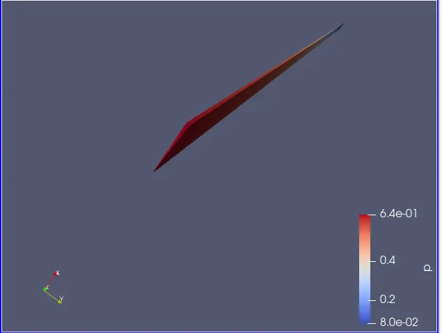
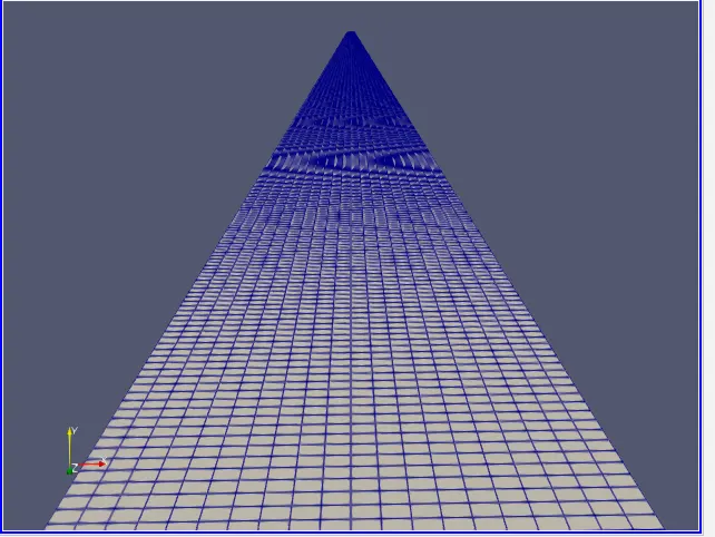
In the paraview once our geometry is loaded it should look like this.
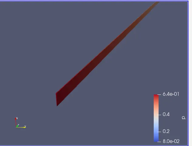
The mesh
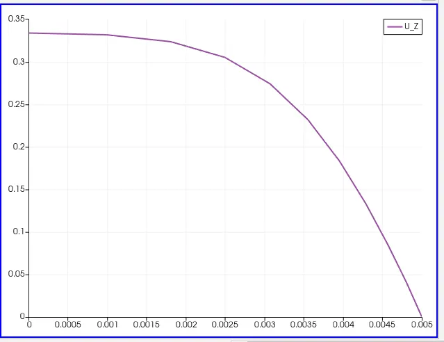
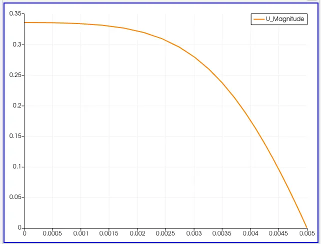
After running the simulation the velocity profile would look like this. We used the plot over line tool in paraview to plot at the required location.
velocity profile for 2 deg wedge at 1.26m
 '
'
Velocity profile for 3 deg wedge at 1.26m
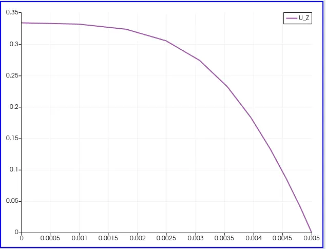
Velocity profile for 4 deg wedge at 1.26m
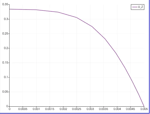
Velocity profile for 4 deg wedge at 1.26m when the number of volumes is doubled in x,z directions
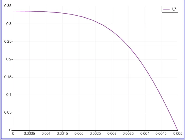
Velocity profile for 4 deg wedge at 1m when the number of volumes is doubled in x,z directions
To calculate the shear stress we use the calculator tool in paraview to calculate the gradients and then multiply the gradients with mu to get the shear stress. The generated shear stress plot would look like this.
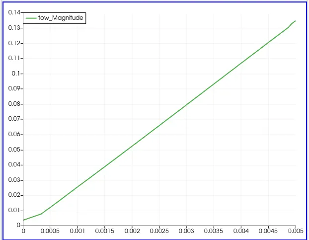
The above plot is generated for 4 deg wedge angle
CONCLUSION
| Velocity Max | 0.374m/s (analytical) | 0.345m/s (simulated) |
| Shear Stress Max | 0. 134174 N/m2 (analytical) | 0.135 N/m2 (simulated) |
- From the above velocity profiles, it can be observed that the velocity profile obtained matches the theoretical profile. Hence the simulation ran successfully with fewer errors.
- The shear stress profile has less magnitude at the center and more magnitude at the walls and then reduces again. This is because due to viscosity the fluid particles at the wall slow down and due to this more shear is produced near the walls. But at the wall fluid particles are at rest hence some shear is reduced.
- The solution seems to be grid-independent as we changed the grid size and still obtained the same results.
The above project can be improved a lot to meet the accuracy. The automation of blockMeshDict file can be done more efficiently.
References have been taken from Wikipedia, Cengel Fluid Mechanics, FM white Fluid Mechanics