Week 11 - Simulation of Flow through a pipe in OpenFoam
AIM:
- To write a program in Matlab that can generate the computational mesh automatically for any wedge angle and grading schemes for an axisymmetric cylindrical pipe.
- To validate the velocity profile with the analytical results using Hagen poiseuille's equation.
THEORY:
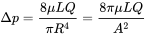
The Hagen–Poiseuille equation, is a physical law that gives the pressure drop in an incompressible and Newtonian fluid in laminar flow flowing through a long cylindrical pipe of constant cross section. The drop in pressure is given by the formula:
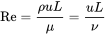
Reynolds number is an important dimensionless quantity in fluid mechanics that determines the flow patterns. At low Reynolds numbers, flows tend to be dominated by laminar flow, while at high Reynolds numbers flows tend to be turbulent. The turbulence results from differences in the fluid's speed and direction, which may sometimes intersect or even move counter to the overall direction of the flow. The reynolds number is given as:
Pressure loss in the pipe:
In the analysis of piping systems, pressure losses are commonly expressed in terms of the equivalent fluid column height, called the head loss hL
hL = ΔPl/ρg
ASSUMPTOINS and PARAMETERS DURING THE STUDY:
1) A wedge section of the entire cylindrical pipe is assumed since the study is axisymmetric. This will greatly save on the computation time required to simulate this problem. Application in pairs to 2-D rotationally symmetric cases to represent planes in the swirl direction.
2)Since the flow is assumed to be incompressiable, viscous and laminar nature, we choose the icofoam solver since it is easy to use and modify, to suit our needs.
3) Pipe diameter = 0.02 m, wedge angle =4, reynolds number = 2100, kinematic viscosity = 0.000001 m^2/s.
The MATLAB code to modify the blockMeshDict file to define the vertices according to the user defined wedge angle is given below:
clear all
close all
clc

re=2100;
d=0.02;
r=d/2;
theta= input('enter the value of theta angle (preferably less than 5 degrees)');
l_e=0.06*re*d; % entry length
l=l_e+0.5;
h=r*sind(theta/2);
v=r*cosd(theta/2);
%finding the vertices
v0=[0 0 0];
v1=[-h v 0];
v2=[h v 0];
v3=[0 0 l];
v4=[-h v l];
v5=[h v l];

f= fopen('blockMeshDict.txt','w');

fprintf(f,'%sn','/*--------------------------------*- C++ -*----------------------------------*');
fprintf(f,'%sn','  =========                 |');
fprintf(f,'%sn','  \      /  F ield         | OpenFOAM: The Open Source CFD Toolbox');
fprintf(f,'%sn','   \    /   O peration     | Website:  https://openfoam.org');
fprintf(f,'%sn','    \  /    A nd           | Version:  8');
fprintf(f,'%sn','     \/     M anipulation  |');
fprintf(f,'%sn','*---------------------------------------------------------------------------*/');
fprintf(f,'%sn','FoamFile');
fprintf(f,'%sn','{');
fprintf(f,'%sn','    version     2.0;');
fprintf(f,'%sn','    format      ascii;');
fprintf(f,'%sn','    class       dictionary;');
fprintf(f,'%sn','    object      blockMeshDict;');
fprintf(f,'%sn','}');
fprintf(f,'%sn','// * * * * * * * * * * * * * * * * * * * * * * * * * * * * * * * * * * * * * //');
fprintf(f,'%sn','');
fprintf(f,'%sn','convertToMeters 1;');
fprintf(f,'%sn','');
fprintf(f,'%sn','vertices');
fprintf(f,'%sn','(');
fprintf(f,'    (%f %f %f)n',v0(1),v0(2),v0(3));
fprintf(f,'    (%f %f %f)n',v1(1),v1(2),v1(3));
fprintf(f,'    (%f %f %f)n',v2(1),v2(2),v2(3));
fprintf(f,'    (%f %f %f)n',v3(1),v3(2),v3(3));
fprintf(f,'    (%f %f %f)n',v4(1),v4(2),v4(3));
fprintf(f,'    (%f %f %f)n',v5(1),v5(2),v5(3));

fprintf(f,'%sn',');');
fprintf(f,'%sn','');
fprintf(f,'%sn','blocks');
fprintf(f,'%sn','(');
fprintf(f,'%sn','    hex (0 2 1 0 3 5 4 3) (20 1 500) simpleGrading (1 1 1)');
fprintf(f,'%sn',');');
fprintf(f,'%sn','');
fprintf(f,'%sn','edges');
fprintf(f,'%sn','(');
fprintf(f,'%sn','	arc 1 2 (0 0.01 0)');
fprintf(f,'%sn','	arc 4 5 (3 0.01 0)');
fprintf(f,'%sn',');');
fprintf(f,'%sn','');
fprintf(f,'%sn','boundary');
fprintf(f,'%sn','(');
fprintf(f,'%sn','    inlet');
fprintf(f,'%sn','    {');
fprintf(f,'%sn','        type patch;');
fprintf(f,'%sn','        faces');
fprintf(f,'%sn','        (');
fprintf(f,'%sn','            (0 0 1 2)');
fprintf(f,'%sn','        );');
fprintf(f,'%sn','    }');
fprintf(f,'%sn','    outlet');
fprintf(f,'%sn','    {');
fprintf(f,'%sn','        type patch;');
fprintf(f,'%sn','        faces');
fprintf(f,'%sn','        (');
fprintf(f,'%sn','            (3 5 4 3)');
fprintf(f,'%sn','        );');
fprintf(f,'%sn','    }');
fprintf(f,'%sn','    top');
fprintf(f,'%sn','    {');
fprintf(f,'%sn','        type wall;');
fprintf(f,'%sn','        faces');
fprintf(f,'%sn','        (');
fprintf(f,'%sn','            (1 4 5 2)');
fprintf(f,'%sn','        );');
fprintf(f,'%sn','    }');
fprintf(f,'%sn','    wedge1');
fprintf(f,'%sn','    {');
fprintf(f,'%sn','        type wedge;');
fprintf(f,'%sn','        faces');
fprintf(f,'%sn','        (');
fprintf(f,'%sn','            (0 2 5 3)');
fprintf(f,'%sn','        );');
fprintf(f,'%sn','    }');
fprintf(f,'%sn','    wedge2');
fprintf(f,'%sn','    {');
fprintf(f,'%sn','        type wedge;');
fprintf(f,'%sn','        faces');
fprintf(f,'%sn','        (');
fprintf(f,'%sn','            (0 3 4 1)');
fprintf(f,'%sn','        );');
fprintf(f,'%sn','    }');
fprintf(f,'%sn','    bot');
fprintf(f,'%sn','    {');
fprintf(f,'%sn','        type empty;');
fprintf(f,'%sn','        faces');
fprintf(f,'%sn','        (');
fprintf(f,'%sn','            (0 0 3 3)');
fprintf(f,'%sn','        );');
fprintf(f,'%sn','    }');
fprintf(f,'%sn',');');
fprintf(f,'%sn','');
fprintf(f,'%sn','mergePatchPairs');
fprintf(f,'%sn','(');
fprintf(f,'%sn',');');
fprintf(f,'%sn','');
fprintf(f,'%sn','// ************************************************************************* //');
The blockMeshDict file is shown below:
/*--------------------------------*- C++ -*----------------------------------*
  =========                 |
  \      /  F ield         | OpenFOAM: The Open Source CFD Toolbox
   \    /   O peration     | Website:  https://openfoam.org
    \  /    A nd           | Version:  8
     \/     M anipulation  |
*---------------------------------------------------------------------------*/
FoamFile
{
    version     2.0;
    format      ascii;
    class       dictionary;
    object      blockMeshDict;
}
// * * * * * * * * * * * * * * * * * * * * * * * * * * * * * * * * * * * * * //

convertToMeters 1;

vertices
(
    (0.000000 0.000000 0.000000)
    (-0.000349 0.009994 0.000000)
    (0.000349 0.009994 0.000000)
    (0.000000 0.000000 3.020000)
    (-0.000349 0.009994 3.020000)
    (0.000349 0.009994 3.020000)
);

blocks
(
    hex (0 2 1 0 3 5 4 3) (20 1 500) simpleGrading (1 1 1)
);

edges
(
	arc 1 2 (0 0.01 0)
	arc 4 5 (3 0.01 0)
);

boundary
(
    inlet
    {
        type patch;
        faces
        (
            (0 0 1 2)
        );
    }
    outlet
    {
        type patch;
        faces
        (
            (3 5 4 3)
        );
    }
    top
    {
        type wall;
        faces
        (
            (1 4 5 2)
        );
    }
    wedge1
    {
        type wedge;
        faces
        (
            (0 2 5 3)
        );
    }
    wedge2
    {
        type wedge;
        faces
        (
            (0 3 4 1)
        );
    }
    bot
    {
        type empty;
        faces
        (
            (0 0 3 3)
        );
    }
);

mergePatchPairs
(
);

// ************************************************************************* //
The outlet initial condition is a fixed value since we assume the pressure at the pipe outlet to be normal air pressure, which is measured as 0. The pressure file is given below:
/*--------------------------------*- C++ -*----------------------------------*
  =========                 |
  \      /  F ield         | OpenFOAM: The Open Source CFD Toolbox
   \    /   O peration     | Website:  https://openfoam.org
    \  /    A nd           | Version:  8
     \/     M anipulation  |
*---------------------------------------------------------------------------*/
FoamFile
{
    version     2.0;
    format      ascii;
    class       volScalarField;
    object      p;
}
// * * * * * * * * * * * * * * * * * * * * * * * * * * * * * * * * * * * * * //

dimensions      [0 2 -2 0 0 0 0];

internalField   uniform 0;

boundaryField
{
    inlet
    {
        type            zeroGradient;
    }

    outlet
    {
        type            fixedValue;
        value		uniform 0;
    }

    top
    {
        type            zeroGradient;
    }
    wedge1
    {
        type            wedge;
    }
    wedge2
    {
        type            wedge;
    }
    bot
    {
        type 		empty;
    }
}

// ************************************************************************* //
The velocity file is given below:
/*--------------------------------*- C++ -*----------------------------------*
  =========                 |
  \      /  F ield         | OpenFOAM: The Open Source CFD Toolbox
   \    /   O peration     | Website:  https://openfoam.org
    \  /    A nd           | Version:  8
     \/     M anipulation  |
*---------------------------------------------------------------------------*/
FoamFile
{
    version     2.0;
    format      ascii;
    class       volVectorField;
    object      U;
}
// * * * * * * * * * * * * * * * * * * * * * * * * * * * * * * * * * * * * * //

dimensions      [0 1 -1 0 0 0 0];

internalField   uniform (0 0 0);

boundaryField
{
    inlet
    {
        type            fixedValue;
	value 		uniform (0 0 0.1050);
    }

    outlet
    {
        type            zeroGradient;
    }

    top
    {
        type            noSlip;
    }
    wedge1
    {
        type            wedge;
    }
    wedge2
    {
        type            wedge;
    }
    bot
    {
        type 		empty;
    }
}

// ************************************************************************* //
The simulation time is considered as 20 seconds and the time step is chosen such that CFL is less than 1. The controlDict file is shown below:
/*--------------------------------*- C++ -*----------------------------------*
  =========                 |
  \      /  F ield         | OpenFOAM: The Open Source CFD Toolbox
   \    /   O peration     | Website:  https://openfoam.org
    \  /    A nd           | Version:  8
     \/     M anipulation  |
*---------------------------------------------------------------------------*/
FoamFile
{
    version     2.0;
    format      ascii;
    class       dictionary;
    location    "system";
    object      controlDict;
}
// * * * * * * * * * * * * * * * * * * * * * * * * * * * * * * * * * * * * * //

application     icoFoam;

startFrom       startTime;

startTime       0;

stopAt          endTime;

endTime         28;

deltaT          0.005;

writeControl    timeStep;

writeInterval   20;

purgeWrite      0;

writeFormat     ascii;

writePrecision  6;

writeCompression off;

timeFormat      general;

timePrecision   6;

runTimeModifiable true;


// ************************************************************************* //
 when calculating the value of dt we must keep in mind that the cfl value <1 thus the value of dt depends on the number of cells we are taking along the z axis and on the x axis. through calculation we have chosen the value of 0.005 which provides a good middle ground between the CFL criterion andthe computational time

 the p file is as shown below

/*--------------------------------*- C++ -*----------------------------------*
  =========                 |
  \      /  F ield         | OpenFOAM: The Open Source CFD Toolbox
   \    /   O peration     | Website:  https://openfoam.org
    \  /    A nd           | Version:  8
     \/     M anipulation  |
*---------------------------------------------------------------------------*/
FoamFile
{
    version     2.0;
    format      ascii;
    class       volScalarField;
    object      p;
}
// * * * * * * * * * * * * * * * * * * * * * * * * * * * * * * * * * * * * * //

dimensions      [0 2 -2 0 0 0 0];

internalField   uniform 0;

boundaryField
{
    inlet
    {
        type            zeroGradient;
    }

    outlet
    {
        type            fixedValue;
        value		uniform 0;
    }

    top
    {
        type            zeroGradient;
    }
    wedge1
    {
        type            wedge;
    }
    wedge2
    {
        type            wedge;
    }
    bot
    {
        type 		empty;
    }
}

// ************************************************************************* //
The MATLAB code to calculate the analytical results and plot the values is given below:
clear all
close all
clc
% reading values from the files
m1= readmatrix('15uR');
u1= m1(:,2);
r1=m1(:,1);

m2= readmatrix('20uR');
u2= m2(:,2);
r2=m2(:,1);

m3= readmatrix('25uR');
u3= m3(:,2);
r3=m3(:,1);

m4= readmatrix('29uR');
u4= m4(:,2);
r4=m4(:,1);


%analytically calculating velocity
for i=1:1001
    if r3(i)>0.01
        u_A(i)=0.210*(1-((r3(i)-0.01)^2/0.01^2));
    else
        u_A(i)=0.210*(1-(((0.01-r3(i))^2)/0.01^2));
    end
end


figure(1)
plot(r1,u1);
hold on
plot(r2,u2);
plot(r3,u3);
plot(r4,u4);
plot(r3,u_A,'linewidth',2);

legend('1.5 meters','2 meters','2.5 meters','2.9 meters','analytical solution')

% shear stress calculation.
u_max=0.210;
re=2100;
r=linspace(0,0.01,1001);
rr1=linspace(0,0.01,1000);
rr=r(2)-r(1);
for i=1:1001
u_A1(i)=0.210*(1-(r(i)^2/0.01^2));
end

ss=0.00089*((abs(diff(u_A1)))/rr);
% ss=flip(ss_tau);
t1= readmatrix('tau');
tau1= t1(:,2);
arc=t1(:,1);

figure(2)
plot(arc,tau1)
hold on
plot(rr1,ss)
legend('from open foam ','analytical values')
RESULTS AND DISCUSSION:
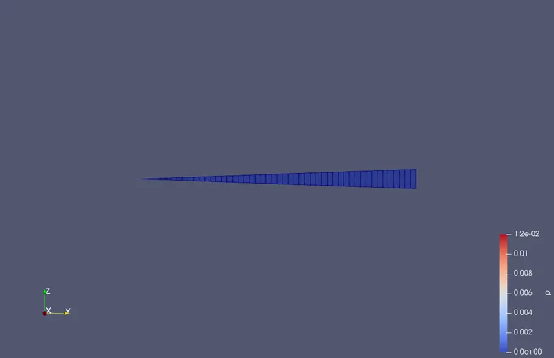
The cross section of the meshed part is shown in the image below:
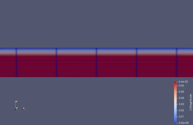
The velocity profiles at t=0, t=5 and t=20 seconds are shown below. Notice that at the boundary surface, the velocity is 0 because of no slip condition and gradually increases towards the center.
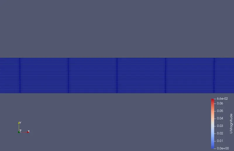
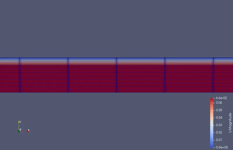
velocity at t=0 velocity at t=5 seconds
The pressure profile and magnitudes are shown below:
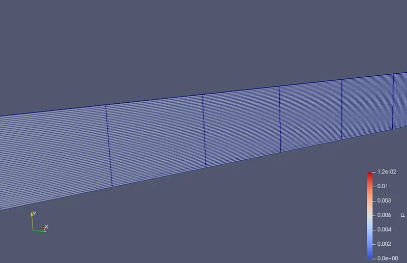
velocity at t=20 seconds.
Validation with the analytical results:
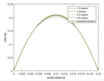
Notice that the velocity increases from 0 to maxium at the center and then becomes zero again ath the boundaries because of no slip condition.
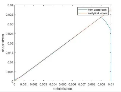
Also the shear stress values are compared from simulation and analytical methods. Notice that the results are accurate.
It is also observed that the velocity profile gradually increases from inlet to the outlet. The velocity reached the maximum value at the outlet and this region is called as a fully developed region as the velocity profile completely developes at the outlet.