Week 11 - Simulation of Flow through a pipe in OpenFoam
Aim: The aim of the challenge is to simulate the flow of fluid across the lenghth of pipe. To compare our analytical result with numerical values for the flow velocity.
Approach: we have considered only the wedge portion of pipe (angle<5) degree for our simulation to reduce the time and effort. We have considered Hagen Poisuellie equation of flow to simuate the results. we have used file praising technique to use the extracted data from paraview so that we can visualize the complete velocity profile and its change at lenght below hydrodynamic length and above hydrodynamic lenghth. Also matlab program is written to generate blockMeshdict file at different wedge angles.
Hagen Poisuellie equation:
The Hagen–Poiseuille equation gives relation between pressure drop flow,radius and viscosity of the fluid.The assumptions of the equation are that the fluid is incompressible and Newtonian; the flow is laminar through a pipe of constant circular cross-section that is substantially longer than its diameter.
Laminar flow:
When a fluid is flowing through a closed channel such as a pipe or between two flat plates, either of two types of flow may occur depending on the velocity and viscosity of the fluid: laminar flow or turbulent flow. Laminar flow occurs at lower velocities, below a threshold at which the flow becomes turbulent. The velocity is determined by a dimensionless parameter characterizing the flow called the Reynolds number, which also depends on the viscosity and density of the fluid and dimensions of the channel.
Reynolds number Re is written as
Re = DVρ/μ
Hydrodynamic Entrance Length:
The hydrodynamic entrance region refers to the area of a pipe where fluid entering a pipe develops a velocity profile due to viscous forces propagating from the interior wall of a pipe.This region is characterized by a non-uniform flow.The fluid enters a pipe at a uniform velocity, then fluid particles in the layer in contact with the surface of the pipe come to a complete stop due to the no slip boundary condition. Due to viscous forces within the fluid, the layer in contact with the pipe surface resists the motion of adjacent layers and slows adjacent layers of fluid down gradually, forming a velocity profile.For the law of conservation of mass to hold true, the velocity of layers of the fluid in the center of the pipe increases to compensate for the reduced velocities of the layers of fluid near the pipe surface. This develops a velocity gradient across the cross section of the pipe.
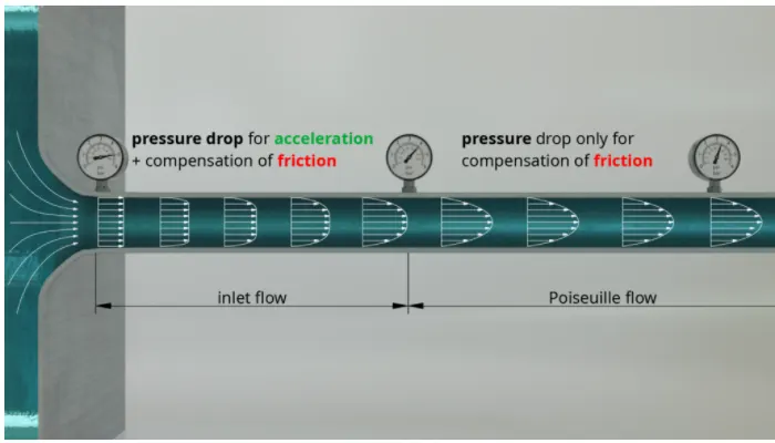
The above figure shows the flow profile changing as flow approaches the lenghth at which it flow becomes stabel and shows a parabolic curve that is the velocity at the centre is max and at the walls is almost zero.The inlet flow region is the hydrodunamic length and poiseuile flow region is the fully developed region of flow.
Formulaes:
Entrance length for laminar flow
Le=0.06*Re*D
Total length of pipe
Lt=Le+0.5 (assusmed)
Reynolds number for laminar flow:
Re=2100
Knimatic viscosity for the fluid (water)
nu=0.89e-6 m^2/s
Dynamic viscosity
mu=0.89e-3 pa.s
Density of water=1000 kg/m^3
Daimeter of pipe=D=0.02 m
radius of pipe=r =0.01 m
Average velocity is calculated by using Reynolds number formula
Re = DVρ/μ
V=Re*nu/D
Vavg=0.093
The maximum velocity is computed by
Vmax=2*Vavg
Vmax=2*0.093=0.1869 m/s
Le=0.06*2100*0.02=2.52 m
Lt=2.52+0.5=3.02 m
Matlab program:The below is the matlab program to generate blockMeshdict file.
clear all
close all
clc
%considered values
theta=4;
d=0.02;%in meters
r=0.01;%in meters
Re=2100;% reynolds number
L_e=Re*d*0.06;%hydrodynamic length of pipe
L_t=L_e+0.5;%total length of pipe
roh=997;%density of water
mu=0.00089;%dynamic viscosity of water

v_avg=(Re*mu)/(roh*d);
v_max=2*(v_avg);
delta_p=(8*mu*L_t*v_avg)/(r^2);
kinematic_p=(delta_p)/(roh);

%shear stress
R=linspace(0,r,1000);
for i=1:length(R)
    tau(i)=2*mu*v_max*(abs(R(i)))/(r^2);
    end
plot(R,tau)
xlabel('radius');
ylabel('shear_stress')

f1=fopen('blockMeshDict','w')

fprintf(f1,'%s','/*--------------------------------*- C++ -*----------------------------------*\');
fprintf(f1,'\n=========            |\n');
fprintf(f1, '\\\\      / F ield        | OpenFOAM: The Open Source CFD Toolbox\n');
fprintf(f1, ' \\\\    /  O peration    | Website: https://openfoam.org\n');
fprintf(f1, '  \\\\  /   A nd          | Version: 8\n');
fprintf(f1, '   \\\\/    M anipulation |\n');
fprintf(f1,'%s','\*---------------------------------------------------------------------------*/');
fprintf(f1,'\nFoamFile\n');
fprintf(f1,'\n{\n');
fprintf(f1,'version 2.0;\n');
fprintf(f1,'format ascii;\n');
fprintf(f1,'class dictionary;\n');
fprintf(f1,'object blockMeshDict;\n');
fprintf(f1,'\n}\n');
fprintf(f1,'%s','// * * * * * * * * * * * * * * * * * * * * * * * * * * * * * * * * * * * * * //');

fprintf(f1,'\n\n convertToMeters 1;\n\n');

%vertices
fprintf(f1,'vertices\n');
fprintf(f1,'(\n');
fprintf(f1,'\t(%d %d %d)\n',0,0,0);
fprintf(f1,'\t(%d %d %d)\n',0,r*cosd(theta/2),-r*sind(theta/2));
fprintf(f1,'\t(%d %d %d)\n',0,r*cosd(theta/2),r*sind(theta/2));
fprintf(f1,'\t(%d %d %d)\n',L_t,0,0);
fprintf(f1,'\t(%d %d %d)\n',L_t,r*cosd(theta/2),-r*sind(theta/2));
fprintf(f1,'\t(%d %d %d)\n',L_t,r*cosd(theta/2),r*sind(theta/2));
fprintf(f1,');\n');

%block
fprintf(f1,'\nblocks\n');
fprintf(f1,'(\n');
fprintf(f1,'\t hex (0 1 2 0 3 4 5 3) (50 1 100) simpleGrading (0.2 1 1)');
fprintf(f1,'\n\n);\n\n');

%edges
fprintf(f1,'edges\n')
fprintf(f1,'(\n')
fprintf(f1,'\t arc %d %d (%d %d %d)\n',1,2,0,r,0);
fprintf(f1,'\t arc %d %d (%d %d %d)\n',4,5,L_t,r,0);
fprintf(f1,'\n\n);\n\n')

%boundary
fprintf(f1,'boundary\n');
fprintf(f1,'(\n');
%inlet
fprintf(f1,'\t inlet\n');
fprintf(f1,'\t{\n');
fprintf(f1,'\t\t type patch;\n');
fprintf(f1,'\t\t faces\n');
fprintf(f1,'\t\t (\n');
fprintf(f1,'\t\t\t\t(%d %d %d %d)\n',0,2,1,0)
fprintf(f1,'\t\t );\n');
fprintf(f1,'\t}\n');
%outlet
fprintf(f1,'\t outlet\n');
fprintf(f1,'\t{\n');
fprintf(f1,'\t\t type patch;\n');
fprintf(f1,'\t\t faces\n');
fprintf(f1,'\t\t (\n');
fprintf(f1,'\t\t\t\t(%d %d %d %d)\n',3,4,5,3)
fprintf(f1,'\t\t );\n');
fprintf(f1,'\t}\n');
%axis
fprintf(f1,'\t axis\n');
fprintf(f1,'\t{\n');
fprintf(f1,'\t\t type empty;\n');
fprintf(f1,'\t\t faces\n');
fprintf(f1,'\t\t (\n');
fprintf(f1,'\t\t\t\t(%d %d %d %d)\n',0,3,3,0)
fprintf(f1,'\t\t );\n');
fprintf(f1,'\t}\n');
%fixedWall
fprintf(f1,'\t fixedWall\n');
fprintf(f1,'\t{\n');
fprintf(f1,'\t\t type wall;\n');
fprintf(f1,'\t\t faces\n');
fprintf(f1,'\t\t (\n');
fprintf(f1,'\t\t\t\t(%d %d %d %d)\n',1,2,5,4)
fprintf(f1,'\t\t );\n');
fprintf(f1,'\t}\n');
%frontWall
fprintf(f1,'\t frontWall\n');
fprintf(f1,'\t{\n');
fprintf(f1,'\t\t type wedge;\n');
fprintf(f1,'\t\t faces\n');
fprintf(f1,'\t\t (\n');
fprintf(f1,'\t\t\t\t(%d %d %d %d)\n',0,3,5,2)
fprintf(f1,'\t\t );\n');
fprintf(f1,'\t}\n');
%backWall
fprintf(f1,'\t backWall\n');
fprintf(f1,'\t{\n');
fprintf(f1,'\t\t type wedge;\n');
fprintf(f1,'\t\t faces\n');
fprintf(f1,'\t\t (\n');
fprintf(f1,'\t\t\t\t(%d %d %d %d)\n',0,1,4,3)
fprintf(f1,'\t\t );\n');
fprintf(f1,'\t}\n');
fprintf(f1,');\n');
fprintf(f1,'mergePatchPairs\n')
fprintf(f1,'(\n');
fprintf(f1,');\n');
fprintf(f1,'\n// ************************************************************************* //\n')


fclose(f1)
Below is the blockMeshdict file generated for wedge angel 4. The below file is replaced with blockMeshdict file in the system folder of cavity case in openFaom.
/*--------------------------------*- C++ -*----------------------------------*\
=========            |
\\      / F ield        | OpenFOAM: The Open Source CFD Toolbox
 \\    /  O peration    | Website: https://openfoam.org
  \\  /   A nd          | Version: 8
   \\/    M anipulation |
\*---------------------------------------------------------------------------*/
FoamFile

{
version 2.0;
format ascii;
class dictionary;
object blockMeshDict;

}
// * * * * * * * * * * * * * * * * * * * * * * * * * * * * * * * * * * * * * //

 convertToMeters 1;

vertices
(
	(0 0 0)
	(0 0.00999391 -0.000348995)
	(0 0.00999391 0.000348995)
	(3.02 0 0)
	(3.02 0.00999391 -0.000348995)
	(3.02 0.00999391 0.000348995)
);

blocks
(
	 hex (0 1 2 0 3 4 5 3) (50 1 300) simpleGrading (0.2 1 1)

);

edges
(
	 arc 1 2 (0 0.01 0)
	 arc 4 5 (3.02 0.01 0)


);

boundary
(
	 inlet
	{
		 type patch;
		 faces
		 (
				(0 2 1 0)
		 );
	}
	 outlet
	{
		 type patch;
		 faces
		 (
				(3 4 5 3)
		 );
	}
	 axis
	{
		 type empty;
		 faces
		 (
				(0 3 3 0)
		 );
	}
	 fixedWall
	{
		 type wall;
		 faces
		 (
				(1 2 5 4)
		 );
	}
	 frontWall
	{
		 type wedge;
		 faces
		 (
				(0 3 5 2)
		 );
	}
	 backWall
	{
		 type wedge;
		 faces
		 (
				(0 1 4 3)
		 );
	}
);
mergePatchPairs
(
);

// ************************************************************************* //
Initail condition
Velocity(U) file
/*--------------------------------*- C++ -*----------------------------------*\
  =========                 |
  \\      /  F ield         | OpenFOAM: The Open Source CFD Toolbox
   \\    /   O peration     | Website:  https://openfoam.org
    \\  /    A nd           | Version:  8
     \\/     M anipulation  |
\*---------------------------------------------------------------------------*/
FoamFile
{
    version     2.0;
    format      ascii;
    class       volVectorField;
    object      U;
}
// * * * * * * * * * * * * * * * * * * * * * * * * * * * * * * * * * * * * * //

dimensions      [0 1 -1 0 0 0 0];

internalField   uniform (0 0 0);

boundaryField
{
    inlet
    {
        type            fixedValue;
        value           uniform (0.093 0 0);
    }

    outlet
    {
        type            zeroGradient;
    }

    axis
    {
        type            empty;
    }
    fixedWall
    {
        type            noSlip;
    }
    frontWall
    {
        type            wedge;
    }
    backWall
    {
        type            wedge;
    }
}

// ************************************************************************* //
Pressure (Kinematic pressure):p
/*--------------------------------*- C++ -*----------------------------------*\
  =========                 |
  \\      /  F ield         | OpenFOAM: The Open Source CFD Toolbox
   \\    /   O peration     | Website:  https://openfoam.org
    \\  /    A nd           | Version:  8
     \\/     M anipulation  |
\*---------------------------------------------------------------------------*/
FoamFile
{
    version     2.0;
    format      ascii;
    class       volScalarField;
    object      p;
}
// * * * * * * * * * * * * * * * * * * * * * * * * * * * * * * * * * * * * * //

dimensions      [0 2 -2 0 0 0 0];

internalField   uniform 0;

boundaryField
{
    inlet
    {
        type            zeroGradient;
    }

    outlet
    {
        type            fixedValue;
        value           uniform 0;
    }

    axis
    {
        type            empty;
    }
    fixedWall
    {
        type            zeroGradient;
    }
    frontWall
    {
        type            wedge;
    }
    backWall
    {
        type            wedge;
    }
}

// ************************************************************************* //
Kinematic viscosity: Transport file
/*--------------------------------*- C++ -*----------------------------------*\
  =========                 |
  \\      /  F ield         | OpenFOAM: The Open Source CFD Toolbox
   \\    /   O peration     | Website:  https://openfoam.org
    \\  /    A nd           | Version:  8
     \\/     M anipulation  |
\*---------------------------------------------------------------------------*/
FoamFile
{
    version     2.0;
    format      ascii;
    class       dictionary;
    location    "constant";
    object      transportProperties;
}
// * * * * * * * * * * * * * * * * * * * * * * * * * * * * * * * * * * * * * //

     nu              [0 2 -1 0 0 0 0] 0.89e-06;  // Nu of water @ 30 degree celcius
//   nu              [0 2 -1 0 0 0 0] 1e-6;       // Nu of water @ 20 degree celcius
//   nu              [0 2 -1 0 0 0 0] 1.3e-6;   // Nu of water @ 10 degree celcius


// ************************************************************************* //
Controldict:
/*--------------------------------*- C++ -*----------------------------------*\
  =========                 |
  \\      /  F ield         | OpenFOAM: The Open Source CFD Toolbox
   \\    /   O peration     | Website:  https://openfoam.org
    \\  /    A nd           | Version:  8
     \\/     M anipulation  |
\*---------------------------------------------------------------------------*/
FoamFile
{
    version     2.0;
    format      ascii;
    class       dictionary;
    location    "system";
    object      controlDict;
}
// * * * * * * * * * * * * * * * * * * * * * * * * * * * * * * * * * * * * * //

application     icoFoam;

startFrom       startTime;

startTime       0;

stopAt          endTime;

endTime         40;

deltaT          0.01;

writeControl    timeStep;

writeInterval   20;

purgeWrite      0;

writeFormat     ascii;

writePrecision  6;

writeCompression off;

timeFormat      general;

timePrecision   6;

runTimeModifiable true;


// ************************************************************************* //
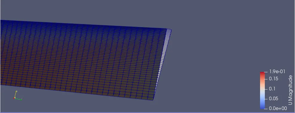
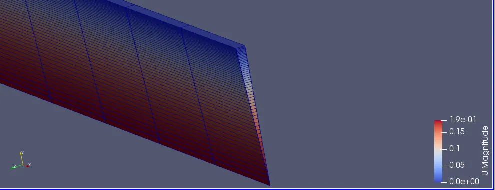
Paraview:
Inlet
Outlet
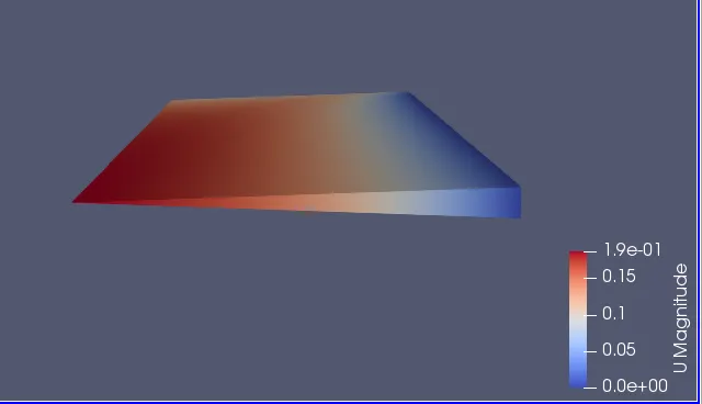
Velocity distribution
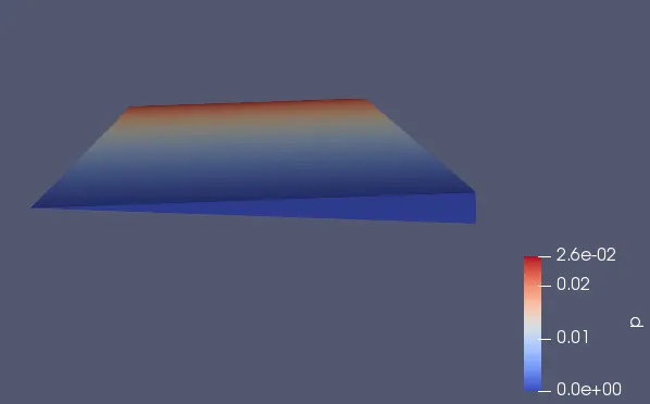
Pressure distribution:
Velocity at different Length of pipe:
Plot over line is used to generate velocity profile at different lenghth of pipe in order to visualize the change in velocity profile as it approaches fully developed velocity profile
Velocity at length 0.1 m
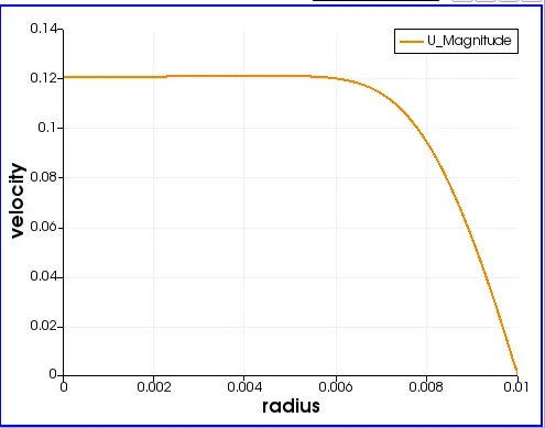
length=1m
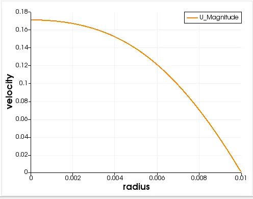
lenght=1.5 m
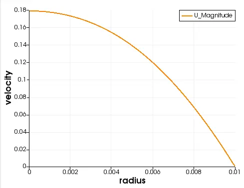
Length=2.52 m
length = 3 m
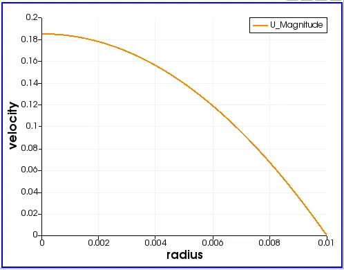
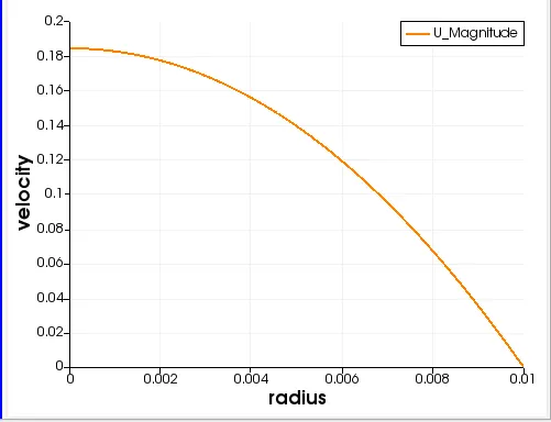
Veocity profile for lenght 2.52 m and length 3 m is same as our hydrodynamic entrance length is 2.52 m as calculated earlier. it shows that our flow has reached fully developed stage as it reached to the lenghth of 2.52 m. in order to visulalize complete plot we have extracted velocity data and arc length at the exit point from paraview in .csv format and copied this data on notepad to convert it into text file. this file is then imported in matlab using file reading. Below is the matlab code to obtain velocity and shear stress.
clear all
close all
clc
f2=fopen('v.txt','r');
fgetl(f2);
A=fscanf(f2,'%f',[3 inf]);
B=A';
mu=0.00089;
U=B(1:end-1,1);
r=B(1:end-1,3);
tau=zeros(length(r));

for i=2:length(r)
tau(i)=mu*((U(i-1)-U(i))/(r(i)-r(i-1)));
end
tau=tau(:,1);
figure(1)
plot(r,tau)
hold on
plot(-r,tau)
xlabel('Radius')
ylabel('Shear stress')
figure(2)
plot(U,r)
hold on
plot(U,-r)
xlabel('Velocity')
ylabel('Radius')
Above matlab program gives follwing plots:
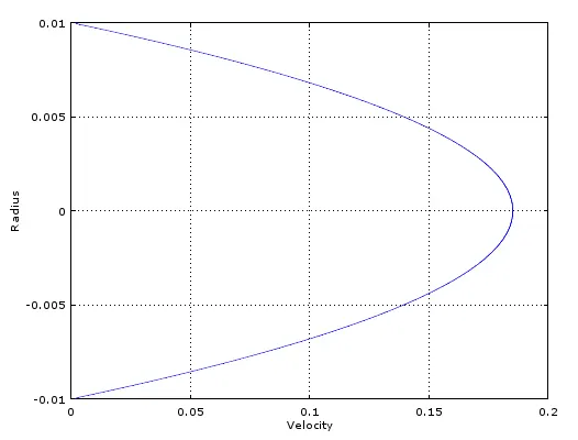
Velocity plot for fully developed flow is parabolic nature as we have considered incompressible newtonian fluid for which velocity is maximum at the centre and decreases due to no slip condition near wall area.Below plot shows velocity profile at length 3 m
Shear stress:
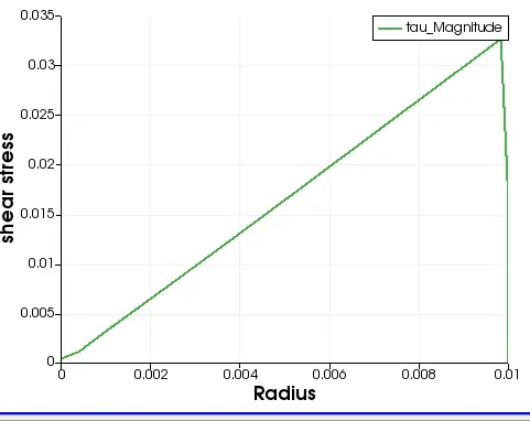
The shear plot shows that maximum shear stress occurs at the wall.In the hydrodynamic entrance region, the wall shear stress is highest at the pipe inlet. Shear stress decreases along the flow direction.That is why the pressure drop is highest in the entrance region of a pipe, which increases the average friction for the whole pipe. This increase in the friction factor is negligible for long pipes.
In fully developed region the pressure gradient and the shear stress in flow are in balance.
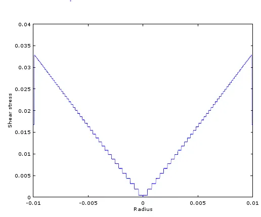
The above shear stress plot is generated by using matlab program but we can also generate shear plot in paraview using plot over line command as shown below is the plot obatained from paraviev.
Result:
| Hagen poisuelle | Simulation value (max velocity) | Error | |
| Velocity | 0.1851 | 0.1869 | 0.0018 |
The Values obtained from simulation and numerically are almost similar.