Week 11 - Simulation of Flow through a pipe in OpenFoam
Aim:
(i)To simulate a transient,axisymmetric laminar flow through the constant cross-section pipe with the reynolds number 2100 using an openFOAM by applying the wedge boundary conditions
(ii)Validating Hydro-dynamic length,fully developed flow velocity profile ,maximum velocity ,pressure drop parameters with the Hagen-poiseuille's equations
(iii)Post-process the shear stress and validate it.
(iv)Generating the blockMeshDict file using an matlab program.
Introduction:
Liquid or gas flow through the pipes is commonly used in heating and cooling applications and Fluid distribution networks.Due to this significant parameter called friction will leads to the pressure drop and head loss, to overcome the pressure drop and headloss ,Pumps (or) fan utilised to flow through the section.Flow sections are circular cross section referred as a pipes. circular cross section withstand large pressure differences between inside and outside without undergoing significant distortion.The primary application of circular cross section pipe is fluid transportation.Non-circular pipes primary application is used for heating and cooling systems of buildings.Circular cross-section pipe has a contact with the fluid particles near the wall,Causes a slight rise in fluid temperature as a result of converting the mechanical energy into the sensible thermal energy then it is said to be frictional heating.Due to the frictional heating the temperature rise in the fluid is negligible.Flow is charcterised by using several parameters among one is reynolds number.Reynolds number is a non-Dimensionalised number and it is defined as ratio of inertial forces to the viscous forces.if reynolds number is less than 2300 then flow is characterised as laminar.Fluid particles present on the laminar flow in a highly ordered fashion (or) Several fluidparticles form as one layer near the wall similar layer has been placed one above the other.If Reynolds number is greater than 4000 then flow is said to be turbulent,turbulent is charecterised as velocity fluctuations and highly disordered motion. If 2300<Re<4000 is a transitional flow,flow changes from completely laminar to completely turbulent,in this region reynolds number depends on the several factors they are geometry,surface roughness,flow velocity,surface temperaure and the type of the fluid.
Reynolds number formula constructed by using the parameters they are (i)Density (ii)Flow velocity (iii) dynamic viscosity of the fluid (iv)characteristic length of the flow section.Flow section may be a circular or non-circular crossection so the characteristic length is the quanity of the hydraulic diameter.Hydraulic diameter is defined as ratio of four times of the area of the crosssection to the wetted perimeter.
Hydraulic diameter is equal to the diameter for the circular cross-section.
on the circular pipe,characterised fluid is entered,if it is a laminar then velocity of the flow near the wall is zero then the friction is transfered from one layer to the another layer.due to this velocity in flow direction increases radial direction,this is clearly explained by the boundary-layer concept. The velocity is zero near the wall because of the no-slip condition and reaches maximum to maintain a constant mass flow rate.velocity is reduced in on layer by bottom layer because of the viscous shearing forces between the layers.if velocity is constant for the layers then viscous effects becomes negligible then it is said tobe irrotational core region. Boundary layer is divided into two categories (i)Velocity boundary layer (ii)Thermal boundary layer.
Velocity Boundary layer where the viscous efffects and velocity changes are importantThe thickness of the boundary layer is defined as distance from the solid wall to the point at which flow velocity is equal to the 99 percent of free stream velocity.At Inlet of pipe,shear stress and pressure drop will be high near the wall as well as newtonian fluids as a constant viscosity and high velocity gradient due to this boundary layer thickness initially will be small,as flow continues shear stress will decreases thickness of the boundary layer increases.Graph will be plotted flow direction velocity vs perpendicular direction cordinates this will provides a velocity profile.This will splits the flow as hydrodynamically developing and developed flow.The velocity profile remains unchanged in the flow direction beyond this region will leads to hydrodynamically developed flow.The hydrodynamically developed flow has a boundary layer near the center from the solid wall.The velociy profile looks like a parabolic curve for the hydrodynamically developed flow.The velocity profile changing in the flow direction is termed as hydrodynamically developing flow.Length of the hydrodynamically developing flow is the hydrodynamic entrance length. Hydrodynamic entry length for laminar flow is determined by using an empirican relation has a two main parameters (i)Reynolds number (ii)Diameter.By considering the sready,laminar,fully developed,incompressible as an Hagen-Poiseuille flow.
Thermal boundary layer develops a fluid at a specified temperature flows over the surface at the different temperature.Temperature profile has developed due to the energy exchanged with the adjacent layer in the direction away (or)normal from the wall and adjacent layer of the surface reaches thermal equlibrium. The thickness of the boundary layer is defined as the distance from the wall to the point, where the temperature difference between the temperature of surface and temperature at that point is equal to the 99% of temperature difference betwen uniform temperature of the fluid and surface temperature of the wall.The adjacent layer of the solid wall where transfers by pure conduction.The convection hear transfer rate anywhere along the surface is directly related to the temperature gradient at that location.
If flow is characterised as turbulent flow ,It is a complex mechanism dominated by fluctuations.Still turbulent on various situations solved based on the experiments (or) empirical (or)semi-empirical relations.Turbulent flow is characterised by the disorderly and rapid fluctuations of swirling regions of fluid called eddies.Swirling eddies will transport mass,momentum and energy as a result of this friction,heat transfer and mass transfer coefficients.Turbulent solved by splitting the instantaneos property into average and fluctuating component.As well as shear stress is higher compared to laminar thats why shear stress is splitted into laminar for the fluid that is near the wall and turbulent for fluid away from the wall,swirling eddies transfer the momentum from a layer to the adjacent layer this is called as reynolds stress and prandtl introduced a mixing length and formulate the turbulent shear stress.turbulent shear stress formulae has formulated like the laminar shear stress formula ,instead of dynamic viscosity ,eddy viscosity is used. Velocity profile obtained for turbulent flow is fuller (or) flat profile.Where velocity profile splits into viscous,buffer,overlap,turbulent layer.based upon this velocity profile differs on each and every layer.Viscous sublayer velocity profile is law of wall where 0<y+<5,Velocity profile cannot able to determine in the buffer layer based on relations 5<y+<30,on the overlap layer,logarithmic law is used for determining the velocity profile 30<Y+<500,turbulent (or) outer layer velocity profile is determined by using velocity defect law. Friction factor is the important parameter in turbulent flow.shear stress and velocity gradient is high near the surface.Hydrodynamic entrance length is 10D.
Matlab Program:
The following script will generate the blockMeshdict file for coarse mesh.obtaining the blockmeshdict file for fine and intermediate mesh by changing the values of no of elements in the direction under the hex block printf line in the script.To change the wedge angles ,after executing the script then line asks for input,wedge angle will change as per the input on the command window.
clear all
close all
clc

%% getting the path of the scipt present on the case folder and creating the path of the blockmeshdict file present under the case/system by using the following commented code
%{
matlabfilePath = matlab.desktop.editor.getActiveFilename;
splitPath=split(matlabfilePath,"/");
Pathlength=length(splitPath);
Pathlength=Pathlength-1;
Joinpath=join(splitPath(1:1:Pathlength),"/")
B='/system/blockMeshDict';
Filepath=string(strcat(Joinpath,B));
%}
%% creating the path for the openfoam file at the current working Directory
Filepath='blockMeshDict';

%% creating the file for the open foam

fileid=fopen(Filepath,'W');
%creating the comment part on the blockMeshDict File
A='/*--------------------------------*- C++ -*----------------------------------*\';
fprintf(fileid,'%s \n',A);
fprintf(fileid,'  =========                 |\n');
fprintf(fileid,'  \\      /  F ield          | OpenFOAM: The Open Source CFD Toolbox\n');
fprintf(fileid,'   \\    /   O peration      | Website:  https://openfoam.org \n');
fprintf(fileid,'    \\  /    A nd            | Version:  10\n');
fprintf(fileid,'     \\/     M anipulation   |\n');
B='\*---------------------------------------------------------------------------*/';
fprintf(fileid,'%s \n',B);
fprintf(fileid,'FoamFile\n{\n    format      ascii;\n    class       dictionary;\n    object      blockMeshDict;\n}\n');
fprintf(fileid,'// * * * * * * * * * * * * * * * * * * * * * * * * * * * * * * * * * * * * * //');
% R=input('dimensions conversion ratio to meter for the geometry')  %conversion ratio from mm (or)cm (or)etc to m
R=1;
fprintf(fileid,'\n\n convertToMeters %f ;\n\n',R);
fprintf(fileid,'vertices \n (\n');
%% Analytical
Wedge_angle=input('Enter the wedge angle');
Reynolds_number=2100;
Density=997.05;               %in kg/m^3
Dynamic_viscosity=0.0008891;    %in kg /m.s
Diameter_of_cylinder=0.02;    %in meters
V_avg=(Reynolds_number*Dynamic_viscosity)/(Density*Diameter_of_cylinder);  % Average Velocity
radius=Diameter_of_cylinder/2;
r=radius;
Length=0.0575*Reynolds_number*Diameter_of_cylinder       % Hydrodynamic length in meters
L=Length+0.405;                                                       %ed on the conversion ratio values on the vertices written on the file
y=(r*(-1)):0.00002:r;                                          %coordinates
v_p=2.*V_avg.*(1-(y.^2./r.^2));                                 %Velocity profile
p_d=(32*Dynamic_viscosity*L*V_avg)/(Diameter_of_cylinder^2);    %Pressure Drop
z=0:0.00282:L;
P_d=(32.*Dynamic_viscosity.*(L-z).*V_avg)./(Diameter_of_cylinder.^2); %pressure Drop profile

tau=(y./2).*(p_d./L);                                           %Shear Stress in the direction

tau =sqrt( tau.^2);
%{
figure('Name','Velocity Profile');
plot(y,v_p)
ylabel('x-directional velocity in m/s')
xlabel('y-cordinates (or)coordinates alomg radius in m')


figure('Name','ShearstressProfile')
plot(y,tau)
xlabel('y-cordinates in m')
ylabel('Shear stress in N/m^2')

figure('Name','PressurDropProfile')
plot(z,P_d)
xlabel('Length cordinates in m')
ylabel('pressure drop in N/m^2')

figure('Name','KinematicPressurDropProfile')
plot(z,P_d/Density)
xlabel('Length cordinates in m')
ylabel('Kinematic pressure drop in m^2/s^2')
%}
%% vertices
a=0;
b=r*cosd(Wedge_angle/2);
c=r*sind(Wedge_angle/2);
e=c*(-1);
fprintf(fileid,'    (%f %f %f)\n',a,a,a);       % Vertices 0
fprintf(fileid,'    (%f %f %f)\n',a,b,c);       % Vertices 1
fprintf(fileid,'    (%f %f %f)\n',a,b,e);       % Vertices 2
fprintf(fileid,'    (%f %f %f)\n',L,a,a);       % Vertices 3
fprintf(fileid,'    (%f %f %f)\n',L,b,c);       % Vertices 4
fprintf(fileid,'    (%f %f %f)\n',L,b,e);       % Vertices 5
fprintf(fileid,');\n\n');
fprintf(fileid,'blocks\n');
fprintf(fileid,'(\n');
fprintf(fileid,'    hex (0 2 1 0 3 5 4 3) (5 1 141) simpleGrading (0.02 1 1)\n);\n\n');
fprintf(fileid,'edges\n(\n');
fprintf(fileid,'    arc 2 1  (0 %f 0)\n',r);
fprintf(fileid,'    arc 5 4  (%f %f 0)\n',L,r);
fprintf(fileid,');\n\n');
fprintf(fileid,'boundary\n');
fprintf(fileid,'(\n');
fprintf(fileid,'    inlet\n    {\n');
fprintf(fileid,'       type patch;\n');
fprintf(fileid,'       faces\n       (\n           (0 1 2 0) \n       );\n    }\n\n');
fprintf(fileid,'    outlet\n    {\n');
fprintf(fileid,'       type patch;\n');
fprintf(fileid,'       faces\n       (\n           (3 5 4 3) \n       );\n    }\n\n');
fprintf(fileid,'    front\n    {\n');
fprintf(fileid,'       type wedge;\n');
fprintf(fileid,'       faces\n       (\n           (0 3 4 1) \n       );\n    }\n\n');
fprintf(fileid,'    Back\n    {\n');
fprintf(fileid,'       type wedge;\n');
fprintf(fileid,'       faces\n       (\n           (0 2 5 3) \n       );\n    }\n\n');
fprintf(fileid,'    axis\n    {\n');
fprintf(fileid,'       type empty;\n');
fprintf(fileid,'       faces\n       (\n           (0 3 3 0) \n       );\n    }\n\n');
fprintf(fileid,'    top\n    {\n');
fprintf(fileid,'       type wall;\n');
fprintf(fileid,'       faces\n       (\n           (1 4 5 2) \n       );\n    }\n);\n\n');
fprintf(fileid,'// ************************************************************************* //');
fclose(fileid);
%% Data generated for pressure,velocity,shear stress

%Pressure
matlabfilePath=pwd;
splitPath=split(matlabfilePath,"/");
Pathlength=length(splitPath);
Pathlength=Pathlength;
Joinpath=join(splitPath(1:1:Pathlength),"/");
B='/data_generated_along_the_line_analytical.csv';
Filepath=string(strcat(Joinpath,B));
g=fopen(Filepath,'W');
C=length(z);
E=P_d./Density;
for c = 1:1:C
    if c == 1
        fprintf(g,'length\tKinematic Pressure\n');
    end

    fprintf(g,'%f \t %f \n',z(c),E(c));
end
fclose(g);

%velocity,shear stress
splitPath=split(matlabfilePath,"/");
Pathlength=length(splitPath);
Pathlength=Pathlength;
Joinpath=join(splitPath(1:1:Pathlength),"/");
B='/data_generated_at_the_line_Analytical.csv';
Filepath=string(strcat(Joinpath,B));
f=fopen(Filepath,'W');
H=length(y);
for h=1:1:H
      if h == 1
        fprintf(f,'radius\tvelocity\tshear stress\n');
    end
    fprintf(f,'%f\t%f\t%f \n',y(h),v_p(h),tau(h));
end
fclose(f);
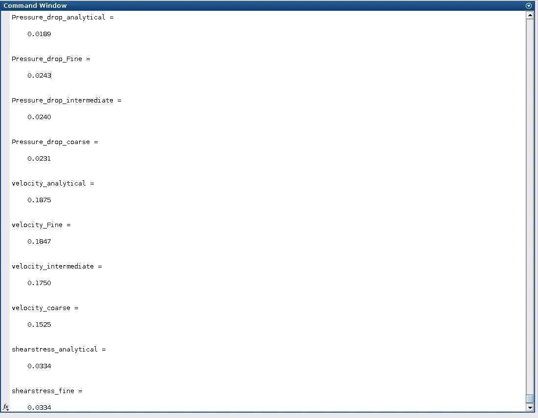
Command window (after execution of script)
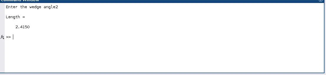
Length represents the hydrodynamic entry length
BlockMeshDict File:
/*--------------------------------*- C++ -*----------------------------------*\
  =========                 |
  \      /  F ield          | OpenFOAM: The Open Source CFD Toolbox
   \    /   O peration      | Website:  https://openfoam.org
    \  /    A nd            | Version:  10
     \/     M anipulation   |
\*---------------------------------------------------------------------------*/
FoamFile
{
    format      ascii;
    class       dictionary;
    object      blockMeshDict;
}
// * * * * * * * * * * * * * * * * * * * * * * * * * * * * * * * * * * * * * //

 convertToMeters 1.000000 ;

vertices
 (
    (0.000000 0.000000 0.000000)
    (0.000000 0.009998 0.000175)
    (0.000000 0.009998 -0.000175)
    (2.820000 0.000000 0.000000)
    (2.820000 0.009998 0.000175)
    (2.820000 0.009998 -0.000175)
);

blocks
(
    hex (0 2 1 0 3 5 4 3) (5 1 141) simpleGrading (0.02 1 1)
);

edges
(
    arc 2 1  (0 0.010000 0)
    arc 5 4  (2.820000 0.010000 0)
);

boundary
(
    inlet
    {
       type patch;
       faces
       (
           (0 1 2 0)
       );
    }

    outlet
    {
       type patch;
       faces
       (
           (3 5 4 3)
       );
    }

    front
    {
       type wedge;
       faces
       (
           (0 3 4 1)
       );
    }

    Back
    {
       type wedge;
       faces
       (
           (0 2 5 3)
       );
    }

    axis
    {
       type empty;
       faces
       (
           (0 3 3 0)
       );
    }

    top
    {
       type wall;
       faces
       (
           (1 4 5 2)
       );
    }
);

// ************************************************************************* //
ControlDict File
/*--------------------------------*- C++ -*----------------------------------*\
  =========                 |
  \\      /  F ield         | OpenFOAM: The Open Source CFD Toolbox
   \\    /   O peration     | Website:  https://openfoam.org
    \\  /    A nd           | Version:  11
     \\/     M anipulation  |
\*---------------------------------------------------------------------------*/
FoamFile
{
    format      ascii;
    class       dictionary;
    location    "system";
    object      controlDict;
}
// * * * * * * * * * * * * * * * * * * * * * * * * * * * * * * * * * * * * * //

application     foamRun;

solver          incompressibleFluid;

startFrom       startTime;

startTime       0;

stopAt          endTime;

endTime         100;

deltaT          0.01;

writeControl    timeStep;

writeInterval   100;

purgeWrite      0;

writeFormat     binary;

writePrecision  6;

writeCompression off;

timeFormat      general;

timePrecision   6;

runTimeModifiable true;

functions
{
    #includeFunc residuals
}


// ************************************************************************* //
fvSolution file:
/*--------------------------------*- C++ -*----------------------------------*\
  =========                 |
  \\      /  F ield         | OpenFOAM: The Open Source CFD Toolbox
   \\    /   O peration     | Website:  https://openfoam.org
    \\  /    A nd           | Version:  10
     \\/     M anipulation  |
\*-------------------------------------------------------------------------*/
FoamFile
{
    format      ascii;
    class       dictionary;
    location    "system";
    object      fvSolution;
}
// * * * * * * * * * * * * * * * * * * * * * * * * * * * * * * * * * * * * * //


solvers
{
    p
    {
        solver          PCG;
        preconditioner  DIC;
        tolerance       1e-06;
        relTol          0.05;
    }

    pFinal
    {
        $p;
        relTol          0;
    }

    U
    {
        solver          smoothSolver;
        smoother        symGaussSeidel;
        tolerance       1e-05;
        relTol          0;
    }
}

PISO
{
    nCorrectors     2;
    nNonOrthogonalCorrectors 0;
    pRefCell        0;
    pRefValue       0;
}


// ************************************************************************* //
fvSchemes file:
/*--------------------------------*- C++ -*----------------------------------*\
  =========                 |
  \\      /  F ield         | OpenFOAM: The Open Source CFD Toolbox
   \\    /   O peration     | Website:  https://openfoam.org
    \\  /    A nd           | Version:  9
     \\/     M anipulation  |
\*---------------------------------------------------------------------------*/
FoamFile
{
    format      ascii;
    class       dictionary;
    object      fvSchemes;
}
// * * * * * * * * * * * * * * * * * * * * * * * * * * * * * * * * * * * * * //

ddtSchemes
{
    default         Euler;
}

gradSchemes
{
    default         Gauss linear;
    grad(p)         Gauss linear;
}

divSchemes
{
    default         none;
    div(phi,U)      Gauss linear;
}

laplacianSchemes
{
    default         Gauss linear orthogonal;
}

interpolationSchemes
{
    default         linear;
}

snGradSchemes
{
    default         orthogonal;
}

}
// ************************************************************************* //
Residuals File:
/*--------------------------------*- C++ -*----------------------------------*\
  =========                 |
  \\      /  F ield         | OpenFOAM: The Open Source CFD Toolbox
   \\    /   O peration     | Website:  https://openfoam.org
    \\  /    A nd           | Version:  11
     \\/     M anipulation  |
-------------------------------------------------------------------------------
Description
    For specified fields, writes out the initial residuals for the first
    solution of each time step; for non-scalar fields (e.g. vectors), writes
    the largest of the residuals for each component (e.g. x, y, z).

\*---------------------------------------------------------------------------*/

#includeEtc "caseDicts/postProcessing/numerical/residuals.cfg"

fields  (p U);

// ************************************************************************* //
physicalProperties File:
/*--------------------------------*- C++ -*----------------------------------*\
  =========                 |
  \\      /  F ield         | OpenFOAM: The Open Source CFD Toolbox
   \\    /   O peration     | Website:  https://openfoam.org
    \\  /    A nd           | Version:  11
     \\/     M anipulation  |
\*---------------------------------------------------------------------------*/
FoamFile
{
    format      ascii;
    class       dictionary;
    location    "constant";
    object      physicalProperties;
}
// * * * * * * * * * * * * * * * * * * * * * * * * * * * * * * * * * * * * * //

transportModel   Newtonian;

nu              [0 2 -1 0 0 0 0] 0.8917e-06;


// ************************************************************************* //
P file:
/*--------------------------------*- C++ -*----------------------------------*\
  =========                 |
  \\      /  F ield         | OpenFOAM: The Open Source CFD Toolbox
   \\    /   O peration     | Website:  https://openfoam.org
    \\  /    A nd           | Version:  11
     \\/     M anipulation  |
\*---------------------------------------------------------------------------*/
FoamFile
{
    format      ascii;
    class       volScalarField;
    object      p;
}
// * * * * * * * * * * * * * * * * * * * * * * * * * * * * * * * * * * * * * //

dimensions      [0 2 -2 0 0 0 0];

internalField   uniform 0;

boundaryField
{
    outlet
    {
       type             fixedValue;
       value            uniform  0;
    }
    inlet
    {
      type              zeroGradient;
    }

    top
    {
        type            zeroGradient;
    }

    front
    {
        type            wedge;
    }

    Back
    {
        type            wedge;
    }
    axis
    {
        type            empty;
    }
}

// ************************************************************************* //
U File:
/*--------------------------------*- C++ -*----------------------------------*\
  =========                 |
  \\      /  F ield         | OpenFOAM: The Open Source CFD Toolbox
   \\    /   O peration     | Website:  https://openfoam.org
    \\  /    A nd           | Version:  11
     \\/     M anipulation  |
\*---------------------------------------------------------------------------*/
FoamFile
{
    format      ascii;
    class       volVectorField;
    object      U;
}
// * * * * * * * * * * * * * * * * * * * * * * * * * * * * * * * * * * * * * //

dimensions      [0 1 -1 0 0 0 0];

internalField   uniform (0 0 0);

boundaryField
{
    inlet
    {
        type           fixedValue;
        value          uniform (0.0937 0 0);
    }
    outlet
    {
        type           zeroGradient;
    }
    front
    {
        type            wedge;
    }
    Back
    {
        type            wedge;
    }
    top
    {
        type            noSlip;
     }

    axis
    {
        type            empty;
    }
}

// ************************************************************************* //
Procedure:
1.copied a case from the icoFoam tutorials to the Desktop and then edited a files to capture the physics as per problem and then files is displayed above.
2.on the terminal,navigate to the case folder.
3. ./Allrun is entered in the terminal and then executed.
4. paraFoam is entered in the terminal and then executed.
5.Apply button is clicked then filters->search->reflect is selected
6.properties->plane->Ymin is selected and then apply button is selected.
7.click calculator and result name is edited then mag(U) is entered then click apply
8.filters->search->gradient then scalar array is selected and then compute gradient box is selected then click apply
9.calculator is selected then result array name is edired then `0.0008891*Gradient` is entered then click apply
10.filters->data Analysis->plot over line is selected then coordinates is entered then click apply and then once again is repeated.
(i)plot over line2-pressure data over the length
(ii)Plot over line1-velocity and shear stress data over the cross sectional length
11.new layout is created by clicking + symbol then click spreadsheet view then selecting plot over line 1 and then click toggle column visiblity and then deselected some parameters then click export spreadsheet option then export view window appears then enter the filename then click ok
selected parameters are points ,shear stress and velocity
12.change plot over line 1 to 2 then click toggle colum visiblity and then deselect parameters and then click export spreadsheet option and then export vire window appears the enter the filename then click ok.
selected parameters are points,pressure
13.foamMonitor -l postProcessing/residuals/0/residuals.dat & is entered in the terminal then using snipping tool plot is captured.
14.From 1 to 13 steps would be repeated for different meshes and for different wedge angles.
Mesh size has been changed by changing the no of cells in each direction under the blocks line present in the matlab script and to carry out the simulations timestep has to be changed as per CFL number.
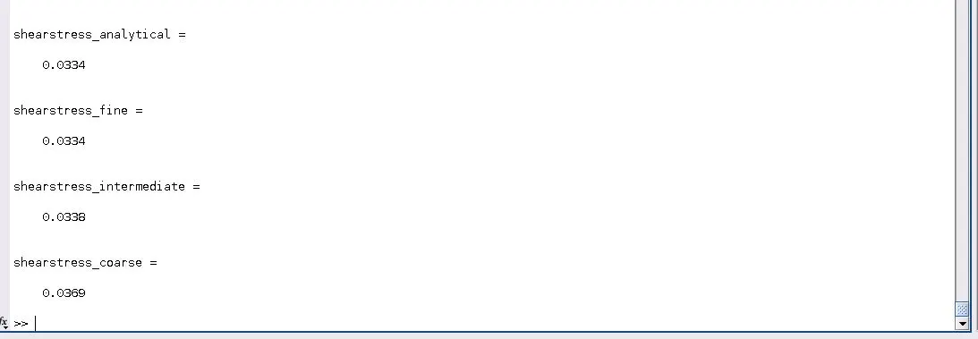
| S.no | Total No.of.cells | no of cells in each direction described on the block mesh dict file | timestep | maximum velocity | maximum shear stress | pressure drop |
| 1. | 705 | (5 1 141) | 0.01 | 0.1525 | 0.0369 | 0.0231 |
| 2. | 2820 | (10 1 282) | 0.008 | 0.1750 | 0.0338 | 0.0240 |
| 3. | 16920 | (30 1 564) | 0.005 | 0.1847 | 0.0334 | 0.0243 |
| 4. | Analytical | 0.1875 | 0.0334 | 0.0189 |
15.Matlab scripts used to plot the comparisions of parameters such as velocity,shearstress and pressure.opened the scripts on the matab and clicked run .it gives figures
scripts are placed outside the case folder,analytical data files kept inside the system,simulation data files kept inside the casefolder/simulation
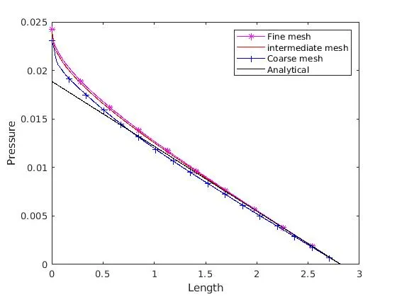
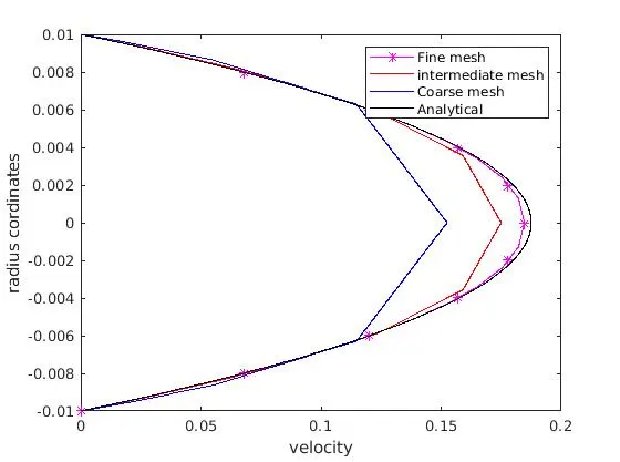
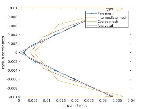
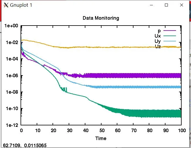
1.coarse Mesh residual plot
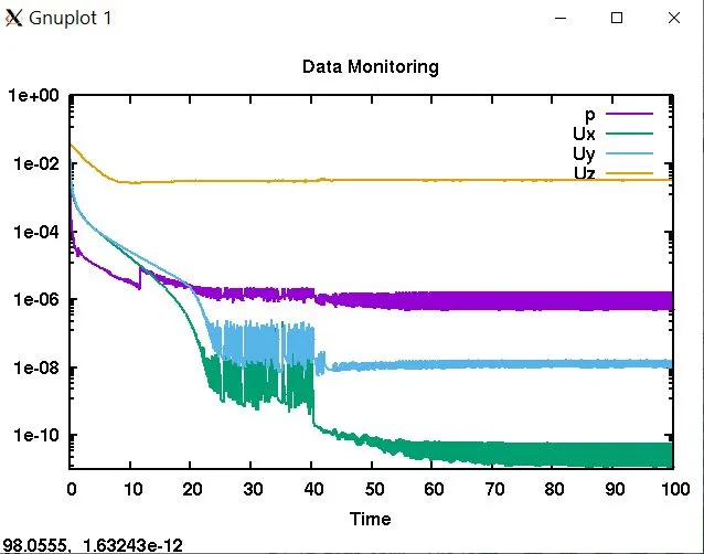
2.Intermediate mesh Residual plot
3.Fine mesh residual plot
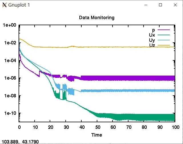
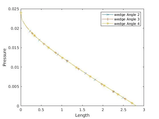
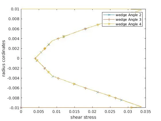
For wedge comparision ,created a different wedge angle by giving an input to the blockmeshdict file generated by matlab script
for comparision of data script placed outside the case folder and case folder/simulation data files placed in this location
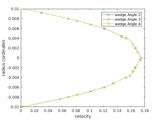
Comparing velocity profile for hydrodynamic length.This is obtained from paraFoam by plotting the multiple location velocity profiles.
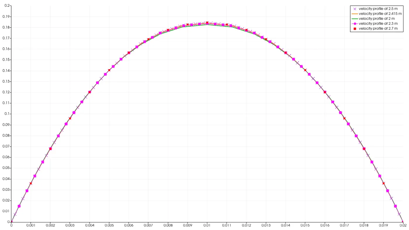
x-axis-radius coedinates
y-axis-velocity
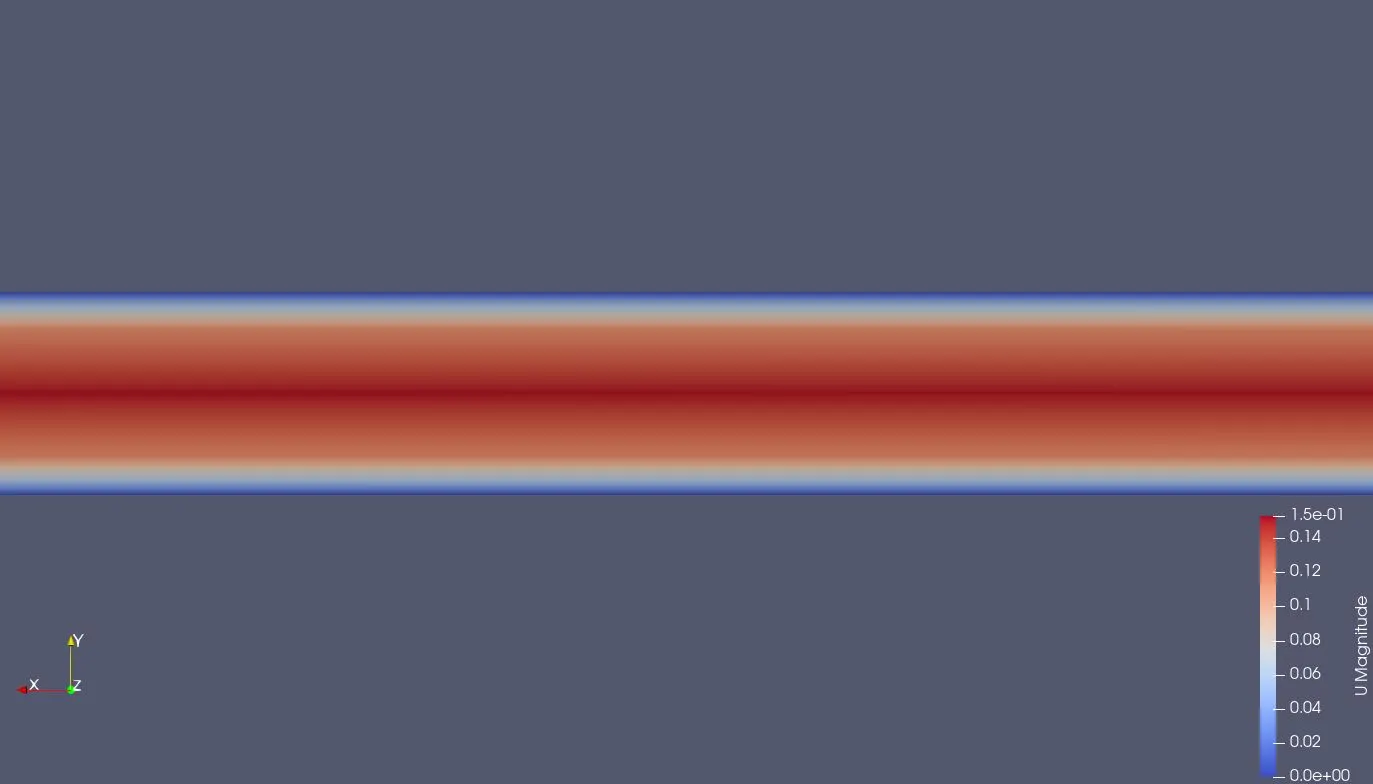
Velocity at the symmetric pipe wedge looks like
Conclusion:
(i) Initial residuals of coarse mesh will become stable faster when compared to the finer mesh.
(ii)Finer mesh will be providing good accuracy for velocity and shear stress parameters but for pressure it is overpredicting
(iii)2,3,4 degrees wedge of the pipe is compared,In plot there is no noticeable difference in the parameters
(iv)As per formula,hydrodynamic entry length is 2.415 m.After simulating the case,plot the velocity profile at different lengths,from that velocity profile after the length of 2.415 m looks similar ,less than 2.415 m has the noticeable difference on velocity profile.
(v)velocity profile is same we can say it as fully developed flow.
Attached the case folder in Zip format:https://drive.google.com/file/d/1P2rXS6r2Fvxc1TuUgNxk_k4sC_FQ5meQ/view?usp=sharing