Week 11 - Simulation of Flow through a pipe in OpenFoam
Simulation of Flow through a pipe in OpenFoam
Aim:-
To simulate flow through a pipe using OpenFoam and validate the results.
Objective:-
- Validate Hydro-dynamic length with the numerical result
- Validate the fully developed flow velocity profile with its analytical profile
- Validate maximum velocity and pressured drop for fully developed flow
- Post-process Shear stress and validate wall shear stress for fully developed flow
Theory;
Laminar Flow: Laminar flow is common only in cases in which the flow channel is relatively small, the fluid is moving slowly, and its viscosity is relatively high. Oil flow through a thin tube or blood flow through capillaries is laminar. Most other kinds of fluid flow are turbulent except near solid boundaries, where the flow is often laminar, especially in a thin layer just adjacent to the surface. See fluid mechanics.
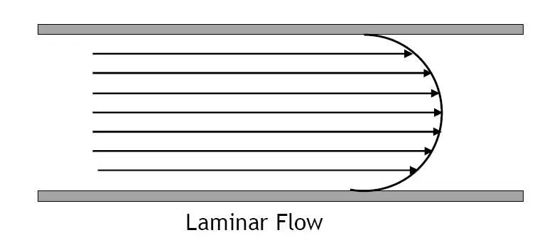
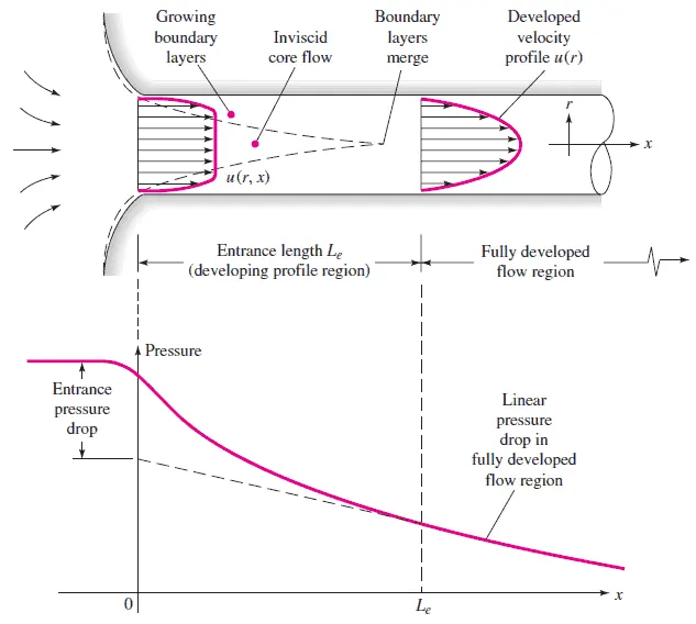
For internal flow regime an entrance region is typical. In this region a nearly inviscid upstream flow converges and enters the tube. To characterize this region the hydrodynamic entrance length is introduced and is approximately equal to:

The maximum hydrodynamic entrance length, at ReD,crit = 2300 (laminar flow), is Le = 138d, where D is the diameter of the pipe. This is the longest development length possible. In turbulent flow, the boundary layers grow faster, and Le is relatively shorter. For any given problem, Le / D has to be checked to see if Le is negligible when compared to the pipe length. At a finite distance from the entrance, the entrance effects may be neglected, because the boundary layers merge and the inviscid core disappears. The tube flow is then fully developed.
Hagen Poisuille's Equation;
The Hagen-Poiseuille equation is used to determine the pressure loss in a steady, hydrodynamically fully-developed, no-swirl flow in a circular pipe. It is given as follows
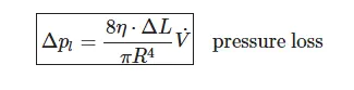
can be rewritten as,
`Deltap = (8*mu*V_(avg)*L)/R^2`
Formula's used in calculation,
`Re = "Inertial Forces"/"Viscous forces"`
`Re = (V_(avg)*D)/nu`
`Re = (rho*V_(avg)*D)/mu`
where Vavg is the average velocity,
nu is the kinematic viscosity
D is the characteristic length of the pipe (diameter)
kinematic viscosity can be defined as the ratio of dynamic viscosity to the density of the fluid.
Assumptions and input parameters,
D = 0.02mm
Re = 2100 for laminar flow
R = D/2
le = 0.05*Re*D = 2.1m
l = 0.3+le = 2.4m
Angle of the wedge (theta) = 3
Defining the properties of the fluid,
Density of the fluid - 997 kg/m3
Dynamic viscosity of the fluid = 0.000890 (N.s/m2)
Average velocity = `V_(avg) = (Re*mu)/(rho*D)` = 9.373e-5 m/s
maximum velocity = `u_max = 2*V_(avg)` = 0.0001875m/s`
pressure drop = `Deltap = (8*mu*V_(avg)*l)/R^2` = 0.000160169
Solving Procedure;
In order to run the simulation in openfoam we require blockmeshDict to generate mesh. To create mesh file we develop a MATLAB code using the input parameters and assuming the wedge profile (parameters) of the pipe.
MATLAB code for Generating blockMeshDict file;
clear all
close all
clc

% Input Parameters

D = 0.02;   %Diameter of the pipe in meters
R = D/2; %Radius of the wedge
Re = 2100;  %Reynolds Number
l_e = 0.05*Re*D;  %Hydrodynamic entry Length
theta = 3;    %Wedge Angle
rho = 997; %kg/m3
mu = 0.00089; %dynamic viscosity
nu = mu/rho; %kinematic iscosity

% Boundary Conditions
v_avg = ((Re*mu)/(rho*D));
v_max = v_avg*2;
l = l_e+0.3; %Total Length
delp = (8*mu*v_avg*l)/(R^2);

scale = 1; %scaling the values to meters

%  Defining the vertices
v0 = [0 0 0];
v1 = [0 R*cosd(theta/2) -R*sind(theta/2)];
v2 = [0 R*cosd(theta/2) R*sind(theta/2)];
v3 = [l 0 0];
v4 = [l R*cosd(theta/2) -R*sind(theta/2)];
v5 = [l R*cosd(theta/2) R*sind(theta/2)];

% Defining blocks and grading factor
cellx = 50; %cell count along x axis
celly = 1;  %cell count along y axis
cellz = 400; %cell count along z axis
gradx = 1; %grading factor along x axis
grady = 1; %grading factor along y axis
gradz = 1; %grading factor along z axis

% Arc Inputs
arc1 = [1,2];
arc2 = [4,5];

% creating the blockMesh structure
f1 = fopen('blockMeshDict.txt','w');
fprintf(f1,'%s\n','/*--------------------------------*- C++ -*----------------------------------*\');
fprintf(f1,'%s\n','========                |');
fprintf(f1,'%s\n','\      /  Field          | OpenFOAM: The Open Source CFD Toolbox');
fprintf(f1,'%s\n',' \    /   O peration     | Website:  https://openfoam.org');
fprintf(f1,'%s\n','  \  /    A nd           | Version:  6');
fprintf(f1,'%s\n','   \/     M anipulation  |');
fprintf(f1,'%s\n',' *---------------------------------------------------------------------------*/');
fprintf(f1,'%s\n','FoamFile');
fprintf(f1,'%s\n','{');
fprintf(f1,'%s\n','    version     2.0;');
fprintf(f1,'%s\n','    format      ascii;');
fprintf(f1,'%s\n','    class       dictionary;');
fprintf(f1,'%s\n','    object      blockMeshDict;');
fprintf(f1,'%s\n','}');
fprintf(f1,'%s\n','// * * * * * * * * * * * * * * * * * * * * * * * * * * * * * * * * * * * * * //');
fprintf(f1,'%s %d %s\n','ConvertToMeters',scale,';');

% Defining Vertices
fprintf(f1,'\n');
fprintf(f1,'%s\n','vertices');
fprintf(f1,'(\n');
fprintf(f1,'     (%d %d %d)\n',v0(1),v0(2),v0(3));
fprintf(f1,'     (%d %d %d)\n',v1(1),v1(2),v1(3));
fprintf(f1,'     (%d %d %d)\n',v2(1),v2(2),v2(3));
fprintf(f1,'     (%d %d %d)\n',v3(1),v3(2),v3(3));
fprintf(f1,'     (%d %d %d)\n',v4(1),v4(2),v4(3));
fprintf(f1,'     (%d %d %d)\n',v5(1),v5(2),v5(3));
fprintf(f1,'%s\n',');');


% Defining Blocks
fprintf(f1,'\n');
fprintf(f1,'%s\n','blocks');
fprintf(f1,'(\n');
fprintf(f1,'hex (0 1 2 0 3 4 5 3)(%d %d %d) %s (%d %d %d)\n',cellx,celly,cellz,'simpleGrading',gradx,grady,gradz);
fprintf(f1,'%s\n',');');

% Defining Edges
fprintf(f1,'\n');
fprintf(f1,'%s\n','edges');
fprintf(f1,'%s\n','(');
fprintf(f1,'   arc %d %d (%d %d %d)\n',arc1(1),arc1(2),0,R,0);
fprintf(f1,'   arc %d %d (%d %d %d)\n',arc2(1),arc2(2),l,R,0);
fprintf(f1,'%s\n',');');

% Defining Boundaries
fprintf(f1,'\n');
fprintf(f1,'%s\n','boundary');
fprintf(f1,'(\n');
fprintf(f1,'   inlet\n');
fprintf(f1,'   {\n');
fprintf(f1,'      type patch;\n');
fprintf(f1,'      faces\n');
fprintf(f1,'      (\n');
fprintf(f1,'          (0 2 1 0)\n');
fprintf(f1,'      );\n');
fprintf(f1,'   }\n');

fprintf(f1,'\n');
fprintf(f1,'   front\n');
fprintf(f1,'   {\n');
fprintf(f1,'      type wedge;\n');
fprintf(f1,'      faces\n');
fprintf(f1,'      (\n');
fprintf(f1,'          (0 3 5 2)\n');
fprintf(f1,'      );\n');
fprintf(f1,'   }\n');

fprintf(f1,'\n');
fprintf(f1,'   back\n');
fprintf(f1,'   {\n');
fprintf(f1,'      type wedge;\n');
fprintf(f1,'      faces\n');
fprintf(f1,'      (\n');
fprintf(f1,'          (0 1 4 3)\n');
fprintf(f1,'      );\n');
fprintf(f1,'   }\n');

fprintf(f1,'\n');
fprintf(f1,'   top\n');
fprintf(f1,'   {\n');
fprintf(f1,'     type wall;\n');
fprintf(f1,'      faces\n');
fprintf(f1,'      (\n');
fprintf(f1,'          (1 2 5 4)\n');
fprintf(f1,'      );\n');
fprintf(f1,'   }\n');

fprintf(f1,'\n');
fprintf(f1,'   axis\n');
fprintf(f1,'   {\n');
fprintf(f1,'     type empty;\n');
fprintf(f1,'      faces\n');
fprintf(f1,'      (\n');
fprintf(f1,'          (0 3 3 0)\n');
fprintf(f1,'      );\n');
fprintf(f1,'   }\n');

fprintf(f1,'\n');
fprintf(f1,'   outlet\n');
fprintf(f1,'   {\n');
fprintf(f1,'      type patch;\n');
fprintf(f1,'      faces\n');
fprintf(f1,'      (\n');
fprintf(f1,'          (3 4 5 3)\n');
fprintf(f1,'      );\n');
fprintf(f1,'   }\n');
fprintf(f1,');\n');
fprintf(f1,'\n');

% Writing the mergepach pairs
fprintf(f1,'%s\n','mergePatchPairs');
fprintf(f1,'(\n');
fprintf(f1,');\n');
fprintf(f1,'%s\n','// ************************************************************************* //');
fclose(f1);
Output of the MATLAB File;
blockMeshDict File;
This can be found in the systm subfolderr of the cavity folder and we need to replace the file with the new file .
/*--------------------------------*- C++ -*----------------------------------*\
========                |
\      /  Field          | OpenFOAM: The Open Source CFD Toolbox
 \    /   O peration     | Website:  https://openfoam.org
  \  /    A nd           | Version:  6
   \/     M anipulation  |
 *---------------------------------------------------------------------------*/
FoamFile
{
    version     2.0;
    format      ascii;
    class       dictionary;
    object      blockMeshDict;
}
// * * * * * * * * * * * * * * * * * * * * * * * * * * * * * * * * * * * * * //
ConvertToMeters 1 ;

vertices
(
     (0 0 0)
     (0 9.996573e-03 -2.617695e-04)
     (0 9.996573e-03 2.617695e-04)
     (2.400000e+00 0 0)
     (2.400000e+00 9.996573e-03 -2.617695e-04)
     (2.400000e+00 9.996573e-03 2.617695e-04)
);

blocks
(
hex (0 1 2 0 3 4 5 3)(50 1 400) simpleGrading (1 1 1)
);

edges
(
   arc 1 2 (0 1.000000e-02 0)
   arc 4 5 (2.400000e+00 1.000000e-02 0)
);

boundary
(
   inlet
   {
      type patch;
      faces
      (
          (0 2 1 0)
      );
   }

   front
   {
      type wedge;
      faces
      (
          (0 3 5 2)
      );
   }

   back
   {
      type wedge;
      faces
      (
          (0 1 4 3)
      );
   }

   top
   {
     type wall;
      faces
      (
          (1 2 5 4)
      );
   }

   axis
   {
     type empty;
      faces
      (
          (0 3 3 0)
      );
   }

   outlet
   {
      type patch;
      faces
      (
          (3 4 5 3)
      );
   }
);

mergePatchPairs
(
);
// ************************************************************************* //
ControlDict;
Here we define the timestep and no of iterations to solve. ControlDict file can be found in the system subfolder of the cavity folder
/*--------------------------------*- C++ -*----------------------------------*\
  =========                 |
  \\      /  F ield         | OpenFOAM: The Open Source CFD Toolbox
   \\    /   O peration     | Website:  https://openfoam.org
    \\  /    A nd           | Version:  10
     \\/     M anipulation  |
\*---------------------------------------------------------------------------*/
FoamFile
{
    format      ascii;
    class       dictionary;
    location    "system";
    object      controlDict;
}
// * * * * * * * * * * * * * * * * * * * * * * * * * * * * * * * * * * * * * //

application     icoFoam;

startFrom       startTime;

startTime       0;

stopAt          endTime;

endTime         0.5;

deltaT          0.0001;

writeControl    timeStep;

writeInterval   10;

purgeWrite      0;

writeFormat     ascii;

writePrecision  6;

writeCompression off;

timeFormat      general;

timePrecision   6;

runTimeModifiable true;


// ************************************************************************* //
Physical Properties,
Here we define the physical properties of the file which is kinematic viscosity in this case and the physical properties file can be found in the constant folder in the cavity1 folder
/*--------------------------------*- C++ -*----------------------------------*\
  =========                 |
  \\      /  F ield         | OpenFOAM: The Open Source CFD Toolbox
   \\    /   O peration     | Website:  https://openfoam.org
    \\  /    A nd           | Version:  10
     \\/     M anipulation  |
\*---------------------------------------------------------------------------*/
FoamFile
{
    format      ascii;
    class       dictionary;
    location    "constant";
    object      physicalProperties;
}
// * * * * * * * * * * * * * * * * * * * * * * * * * * * * * * * * * * * * * //

nu              [0 2 -1 0 0 0 0] 8.93e-7;


// ************************************************************************* //
Field Operations;
For Pressure distribution around the wedge profile,
Here we define the named selection of the geometry and the properties acting on the surfaces.
/*--------------------------------*- C++ -*----------------------------------*\
  =========                 |
  \\      /  F ield         | OpenFOAM: The Open Source CFD Toolbox
   \\    /   O peration     | Website:  https://openfoam.org
    \\  /    A nd           | Version:  10
     \\/     M anipulation  |
\*---------------------------------------------------------------------------*/
FoamFile
{
    format      ascii;
    class       volScalarField;
    object      p;
}
// * * * * * * * * * * * * * * * * * * * * * * * * * * * * * * * * * * * * * //

dimensions      [0 2 -2 0 0 0 0];

internalField   uniform 0;

boundaryField
{
    inlet
    {
        type            zeroGradient;
    }

    front
    {
        type            wedge;
    }

    back
    {
        type            wedge;
    }

    top
    {
        type            zeroGradient;
    }

    axis
    {
        type            empty;
    {

    outlet
    {
        type            fixedValue;
        value           uniform 0;
    }
}

// ************************************************************************* //
For Velocity distribution profile around the wedge,
/*--------------------------------*- C++ -*----------------------------------*\
  =========                 |
  \\      /  F ield         | OpenFOAM: The Open Source CFD Toolbox
   \\    /   O peration     | Website:  https://openfoam.org
    \\  /    A nd           | Version:  10
     \\/     M anipulation  |
\*---------------------------------------------------------------------------*/
FoamFile
{
    format      ascii;
    class       volVectorField;
    object      U;
}
// * * * * * * * * * * * * * * * * * * * * * * * * * * * * * * * * * * * * * //

dimensions      [0 1 -1 0 0 0 0];

internalField   uniform (0.75 0 0);

boundaryField
{
    inlet
    {
        type            fixedValue;
        value           uniform (0.75 0 0);
    }

    front
    {
        type            wedge;
    }

    back
    {
        type            wedge;
    }

    top
    {
        type            noSlip;
    }

    axis
    {

        type            empty;
    }

    outlet
    {
        type            zeroGradient;
    }
}

// ************************************************************************* //
Note: Maintain the same named region for the blockmeshdict and p,U.
Calculation
After setting up the necessary conditions and named selections,
Generate mesh using - blockMesh command
To check the mesh use - checkMesh command
To solve use - icoFoam command to start the calculation . Here we consider the flow as incompressible laminar hence icoFoam is used.
Visualize the Result;
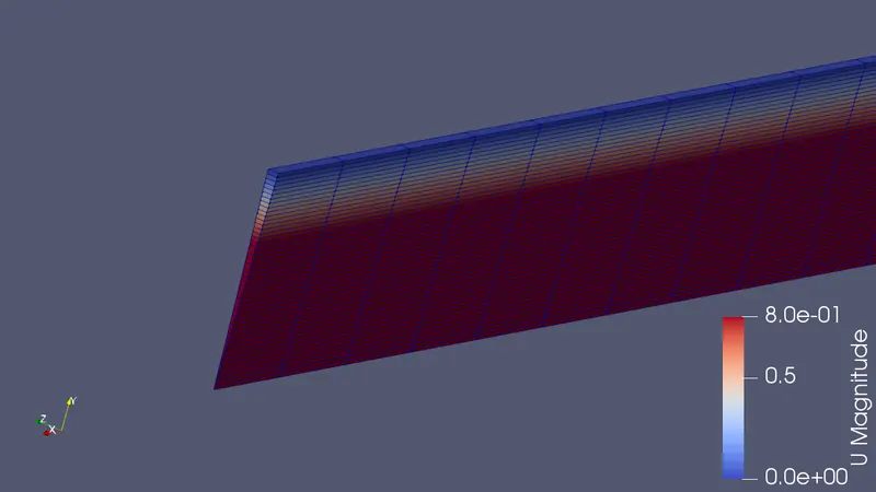
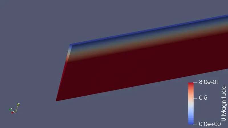
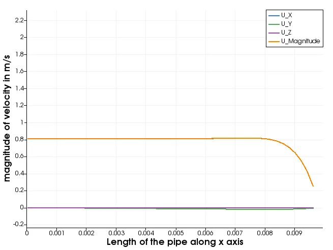
Analyze velocity distribution over random area using points;
use plot over lines in dataaalytics in filter menu
velocity profile near the exit ,
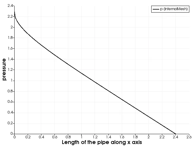
Presssure distribution alon the weedge
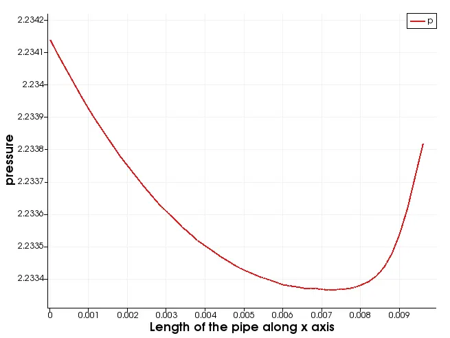
shear stress;
file:///home/sri/Documents/New%20Folder/t%20chart.png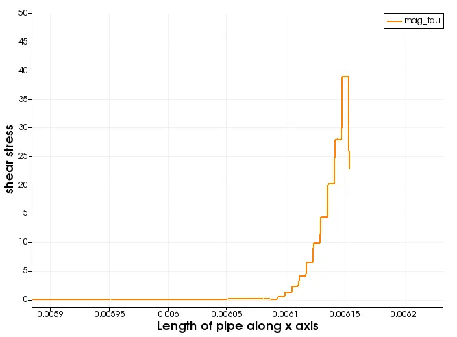
Validating with MATLAB;
clear all
close all
clc

% Required variables
% Reynold's number
D = 0.02;
R = D/2;
R_e = 2100;
L_e = 0.05*R_e*D;
L = 0.3+L_e;
theta = 3;
mu = 0.00089;  % Dynamic viscosity (N.s/m^2)
rho = 997; % (kg/m3)
nu = mu/rho;

% Read the text files extracted from simulation
f1 = fopen('velocity.csv','r');
A = fgetl(f1);
for i = 1:1000
    B = fgetl(f1);
    C = strsplit(B,',');
    vel_n(i) = C(1);
    Len_n(i) = C(3);
end
vel_n = str2double(vel_n');
Len_n = str2double(Len_n');

% Reading and Extracting shear stress
f2 = fopen('shear_stress.csv','r');
A = fgetl(f2);
for i = 1:1000
    B = fgetl(f2);
    C = strsplit(B,',');
    tau_n(i) = C(2);
    Len_n2(i) = C(1);
end
tau_n = str2double(tau_n');
Len_n2 = str2double(Len_n2');

r = linspace(0,R,1000);   % Radial Distance
% Hagen Poiseuille's solution
v_avg = (R_e*mu)/(rho*D); %Average velocity
u_max = 2*v_avg %maximum Velocity
v_r = u_max*(1-(r.^2/R^2))

% Hagen poiseille's Equation for Pressure Drop
P_len = linspace(0,L,1000)
P_len1 = P_len';
for i = 1:length(P_len1)
    delta_p(i) = (8*mu*P_len1(i)*v_avg)/R^2;
    k_pre(i) = delta_p(i)/rho;  %kinematicc pressure
end

k_pre = fliplr(k_pre);

% Analytical shear stress calculation
for i = 1:length(r)
    tau_an(i) = (2*mu*u_max*r(i))/R^2;
    tau_an1=tau_an';
end

figure(1)
plot(r,vel_n,'r','linewidth',1) % Anaytical Data
hold on
plot(Len_n,vel_n,'--','color','k','linewidth',1) % Numerical Data
title('Velocity: Numerical vs Analytical Data')
xlabel('Radial Length (m)')
ylabel('Velocity in m/s')
legend('Analytical Method','Numerical Method')
grid on

figure(2)
plot(r,tau_an1,'b','linewidth',1) % Anaytical Data
hold on
plot(Len_n,tau_n,'--','color','g','linewidth',1) % Numerical Data
title('Velocity: Numerical vs Analytical Data')
xlabel('Radial Length (m)')
ylabel('Velocity in m/s')
legend('Analytical Method','Numerical Method')
grid on
Visualizing the result;
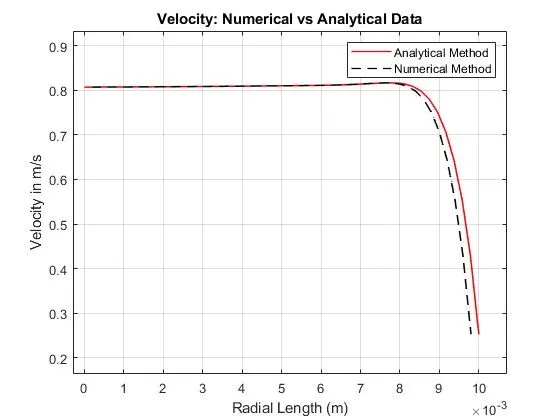
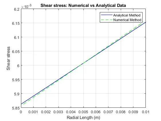
Conclusion:
Simulation of flow through pipe using openFoam is carried and the rsults are validated with MATLAB.