Week 11 - Simulation of Flow through a pipe in OpenFoam
AIM
1. To simulate an axi-symmetric flow by applying the wedge boundary condition that is laminar and flows through a constant cross-section pipe at an inlet Reynold's number of 2100.
2. Also write a code in Matlab to automate the generation of blockMeshDict file by taking inputs like pipe length, diameter, wedge angle, etc and output a fully functional blockMeshDict file.
Expected Results
- Validate Hydro-dynamic length with the numerical result
- Validate the fully developed flow velocity profile with its analytical profile
- Validate maximum velocity and pressured drop for fully developed flow
- Post-process Shear stress and validate wall shear stress for fully developed flow.
EXPLAINATION
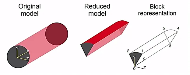
To simulate the incompressible laminar flow through a cylindrical pipe, I have used the icoFoam solver in OpenFoam. Also simulating the flow through an entire pipe would be computationally demanding, and since the geometry of the pipe is axisymmetric I have used a wedge section of pipe for the simulation as depicted in the below figure.
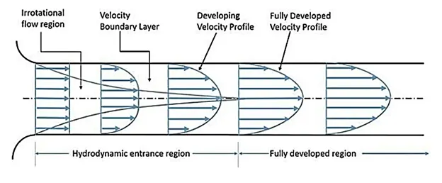
As shown in the above figure, when the fluid enters the pipe, we see viscous effects because of the flow resistance characteristic of the pipe wall. The viscous effects are important at the boundary layer. The boundary layer is a dynamic phenomenon, and it is seen that it grows from the wall to such an extent that they all merge on the centerline of the pipe. That is when the flow is said to be a fully developed flow. The length required for the flow to reach a fully developed flow condition is called the hydrodynamic entrance length denoted by Le.
We have an emperical equation to compute the hydrodynamic entrance length given by
Le = 0.06*Re*D
where, Re = Reynold's number
D = Diameter of the pipe
The velocity profile of a fully developed laminar horizontal circular pipe flow is given by
`V = 1/(4mu)(partialp)/(partialx)(y^2-R^2)`
Similarly we have an equation for pressure difference given by
`deltap = (32muLV)/(D^2)`
where, V = average velocity
mu = dynamic viscosity
y = vertical distance from the pipe axis
Analytical solution is given by Hagen-Poiseuille equations
Average velocity can be computed from the Reynold's number equation i.e., `V = (mu*Re)/(rho*D)`
= (0.001003*2100)/(998.2*0.008)
= 0.2637 m/s
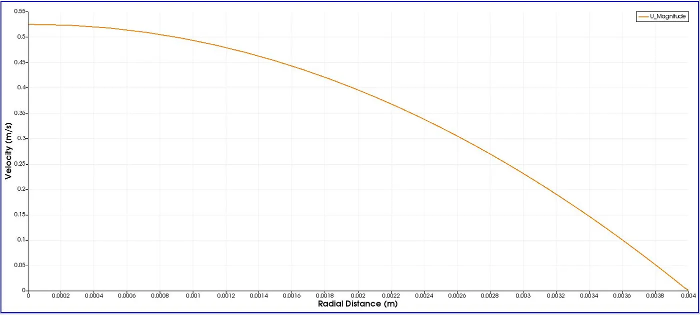
WKT, maximum velocity = 2 * Average velocity. Hence max. velocity = 0.5274 m/s
Hydrodynamic entrance length (Le) = 0.06*Re*D = 0.06*2100*0.008 = 1.008 m
Hence pressure drop in the fully developed flow i.e., from 1.008 to 1.5 m = (32*0.001003*0.4*0.2637)/0.008^2
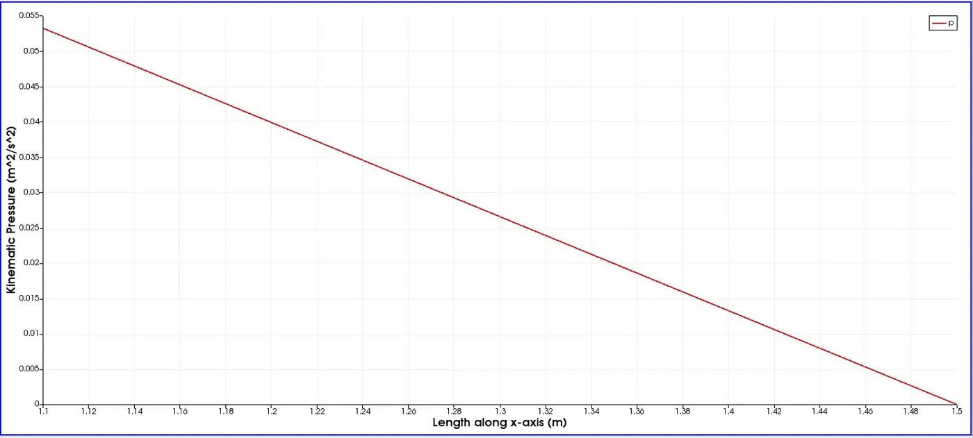
= 52.89 Pa
Note that the solver in the OpenFOAM uses kinematic pressure which is the ratio of Static pressure and density and hence we need to compute the kinematic pressure given by 52.89/998.2 = 0.053 m2/s2
MATLAB code to create a blockMeshDict file
clear all
close all
clc

%Inputs

L=1.5;
r=0.004;
theta=3;
nx=500;
ny=40;
nz=1;

%blockMeshDict
f1=fopen('blockMeshDict','w')

fprintf(f1,'convertToMeters 1;nn');

%Vertices
fprintf(f1,'verticesn');
fprintf(f1,'(n');
fprintf(f1,'t (%d %d %d)n',0,0,0); %Point 0
fprintf(f1,'t (%d %d %d)n',0,r*cosd(theta/2),r*sind(theta/2)); %Point 1
fprintf(f1,'t (%d %d %d)n',0,r*cosd(theta/2),-r*sind(theta/2)); %Point 2
fprintf(f1,'t (%d %d %d)n',L,0,0); %Point 3
fprintf(f1,'t (%d %d %d)n',L,r*cosd(theta/2),r*sind(theta/2)); %Point 4
fprintf(f1,'t (%d %d %d)n',L,r*cosd(theta/2),-r*sind(theta/2)); %Point 5
fprintf(f1,');nn');

%Blocks
fprintf(f1,'blocksn');
fprintf(f1,'(n');
fprintf(f1,'     hex (0 3 5 2 0 3 4 1) (%d %d %d) ',nx,ny,nz);
fprintf(f1,'simpleGrading (1 0.1 1)nn');
fprintf(f1,');nn');

%Edges
fprintf(f1,'edgesn(nt arc %d %d (%d %d %d)n',1,2,0,r,0);
fprintf(f1,'t arc %d %d (%d %d %d)n',4,5,L,r,0);
fprintf(f1,');nn');

%Boundary
fprintf(f1,'boundaryn(n');

fprintf(f1,'t inletn'); %Inlet
fprintf(f1,'t{n');
fprintf(f1,'tt type patch;n');
fprintf(f1,'tt facesn');
fprintf(f1,'tt(n');
fprintf(f1,'ttt (0 1 2 0)n');
fprintf(f1,'tt );n');
fprintf(f1,'t}n');

fprintf(f1,'t outletn'); %Outlet
fprintf(f1,'t{n');
fprintf(f1,'tt type patch;n');
fprintf(f1,'tt facesn');
fprintf(f1,'tt (n');
fprintf(f1,'ttt (3 5 4 3)n');
fprintf(f1,'tt );n');
fprintf(f1,'t}n');

fprintf(f1,'t Noslipwalln'); %Top-Noslipwall
fprintf(f1,'t{n');
fprintf(f1,'tt type wall;n');
fprintf(f1,'tt facesn');
fprintf(f1,'tt (n');
fprintf(f1,'ttt (1 4 5 2)n');
fprintf(f1,'tt );n');
fprintf(f1,'t}n');

fprintf(f1,'t backn'); %Back
fprintf(f1,'t{n');
fprintf(f1,'tt type wedge;n');
fprintf(f1,'tt facesn');
fprintf(f1,'tt (n');
fprintf(f1,'ttt (0 2 5 3)n');
fprintf(f1,'tt );n');
fprintf(f1,'t}n');

fprintf(f1,'t frontn'); %Front
fprintf(f1,'t{n');
fprintf(f1,'tt type wedge;n');
fprintf(f1,'tt facesn');
fprintf(f1,'tt (n');
fprintf(f1,'ttt (0 3 4 1)n');
fprintf(f1,'tt );n');
fprintf(f1,'t}n');

fprintf(f1,'t axisn'); %Axis
fprintf(f1,'t{n');
fprintf(f1,'tt type empty;n');
fprintf(f1,'tt facesn');
fprintf(f1,'tt (n');
fprintf(f1,'ttt (0 3 3 0)n');
fprintf(f1,'tt );n');
fprintf(f1,'t}n');
fprintf(f1,');nn');

fclose(f1);
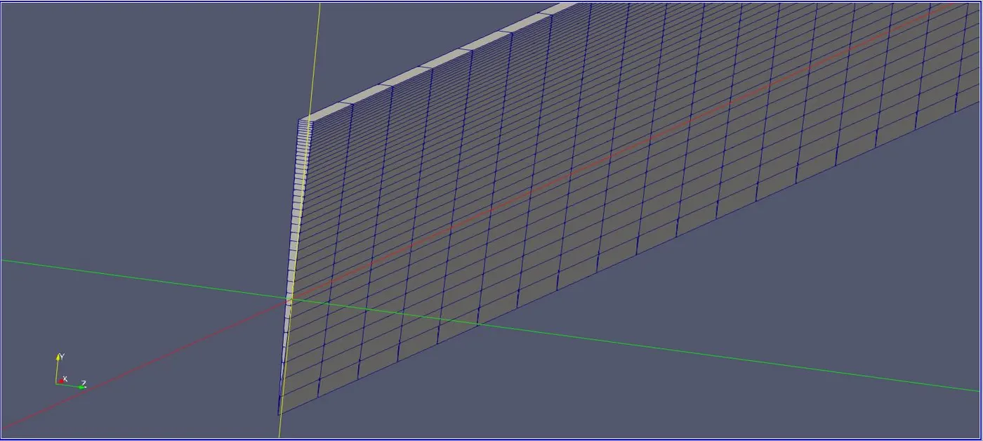
Generated blockMeshDict file and geometry
convertToMeters 1;

vertices
(
	 (0 0 0)
	 (0 3.998629e-03 1.047078e-04)
	 (0 3.998629e-03 -1.047078e-04)
	 (1.500000e+00 0 0)
	 (1.500000e+00 3.998629e-03 1.047078e-04)
	 (1.500000e+00 3.998629e-03 -1.047078e-04)
);

blocks
(
     hex (0 3 5 2 0 3 4 1) (500 40 1) simpleGrading (1 0.1 1)

);

edges
(
	 arc 1 2 (0 4.000000e-03 0)
	 arc 4 5 (1.500000e+00 4.000000e-03 0)
);

boundary
(
	 inlet
	{
		 type patch;
		 faces
		(
			 (0 1 2 0)
		 );
	}
	 outlet
	{
		 type patch;
		 faces
		 (
			 (3 5 4 3)
		 );
	}
	 Noslipwall
	{
		 type wall;
		 faces
		 (
			 (1 4 5 2)
		 );
	}
	 back
	{
		 type wedge;
		 faces
		 (
			 (0 2 5 3)
		 );
	}
	 front
	{
		 type wedge;
		 faces
		 (
			 (0 3 4 1)
		 );
	}
	 axis
	{
		 type empty;
		 faces
		 (
			 (0 3 3 0)
		 );
	}
); 
Initial and boundary conditions
/*--------------------------------*- C++ -*----------------------------------*
  =========                 |
  \      /  F ield         | OpenFOAM: The Open Source CFD Toolbox
   \    /   O peration     | Website:  https://openfoam.org
    \  /    A nd           | Version:  8
     \/     M anipulation  |
*---------------------------------------------------------------------------*/
FoamFile
{
    version     2.0;
    format      ascii;
    class       volVectorField;
    object      U;
}
// * * * * * * * * * * * * * * * * * * * * * * * * * * * * * * * * * * * * * //

dimensions      [0 1 -1 0 0 0 0];

internalField   uniform (0.2637 0 0);

boundaryField
{
    inlet
    {
        type            fixedValue;
        value           uniform (0.2637 0 0);
    }

    outlet
    {
        type            zeroGradient;
    }

    Noslipwall
    {
        type            noSlip;
    }

    back
    {
        type            wedge;
    }

    front
    {
        type            wedge;
    }

    axis
    {
        type            empty;
    }
}

// ************************************************************************* //
/*--------------------------------*- C++ -*----------------------------------*
========= |
\ / F ield | OpenFOAM: The Open Source CFD Toolbox
\ / O peration | Website: https://openfoam.org
\ / A nd | Version: 8
\/ M anipulation |
*---------------------------------------------------------------------------*/
FoamFile
{
version 2.0;
format ascii;
class volScalarField;
object p;
}
// * * * * * * * * * * * * * * * * * * * * * * * * * * * * * * * * * * * * * //
dimensions [0 2 -2 0 0 0 0];
internalField uniform 0;
boundaryField
{
inlet
{
type zeroGradient;
}
outlet
{
type fixedValue;
value uniform 0;
}
Noslipwall
{
type zeroGradient;
}
back
{
type wedge;
}
front
{
type wedge;
}
axis
{
type empty;
}
}
// ************************************************************************* //controlDict file
/*--------------------------------*- C++ -*----------------------------------*
  =========                 |
  \      /  F ield         | OpenFOAM: The Open Source CFD Toolbox
   \    /   O peration     | Website:  https://openfoam.org
    \  /    A nd           | Version:  8
     \/     M anipulation  |
*---------------------------------------------------------------------------*/
FoamFile
{
    version     2.0;
    format      ascii;
    class       dictionary;
    location    "system";
    object      controlDict;
}
// * * * * * * * * * * * * * * * * * * * * * * * * * * * * * * * * * * * * * //

application     icoFoam;

startFrom       startTime;

startTime       0;

stopAt          endTime;

endTime         20;

deltaT          0.001;

writeControl    timeStep;

writeInterval   20;

purgeWrite      0;

writeFormat     ascii;

writePrecision  6;

writeCompression off;

timeFormat      general;

timePrecision   6;

runTimeModifiable true;


// ************************************************************************* //
Physical properties file
/*--------------------------------*- C++ -*----------------------------------*
  =========                 |
  \      /  F ield         | OpenFOAM: The Open Source CFD Toolbox
   \    /   O peration     | Website:  https://openfoam.org
    \  /    A nd           | Version:  8
     \/     M anipulation  |
*---------------------------------------------------------------------------*/
FoamFile
{
    version     2.0;
    format      ascii;
    class       dictionary;
    location    "constant";
    object      transportProperties;
}
// * * * * * * * * * * * * * * * * * * * * * * * * * * * * * * * * * * * * * //

nu              [0 2 -1 0 0 0 0] 1.0048e-06;


// ************************************************************************* //
fvScheme file
/*--------------------------------*- C++ -*----------------------------------*
  =========                 |
  \      /  F ield         | OpenFOAM: The Open Source CFD Toolbox
   \    /   O peration     | Website:  https://openfoam.org
    \  /    A nd           | Version:  8
     \/     M anipulation  |
*---------------------------------------------------------------------------*/
FoamFile
{
    version     2.0;
    format      ascii;
    class       dictionary;
    location    "system";
    object      fvSchemes;
}
// * * * * * * * * * * * * * * * * * * * * * * * * * * * * * * * * * * * * * //

ddtSchemes
{
    default         Euler;
}

gradSchemes
{
    default         Gauss linear;
    grad(p)         Gauss linear;
}

divSchemes
{
    default         none;
    div(phi,U)      Gauss linear;
}

laplacianSchemes
{
    default         Gauss linear orthogonal;
}

interpolationSchemes
{
    default         linear;
}

snGradSchemes
{
    default         orthogonal;
}


// ************************************************************************* //
fvSolution file
/*--------------------------------*- C++ -*----------------------------------*
  =========                 |
  \      /  F ield         | OpenFOAM: The Open Source CFD Toolbox
   \    /   O peration     | Website:  https://openfoam.org
    \  /    A nd           | Version:  8
     \/     M anipulation  |
*---------------------------------------------------------------------------*/
FoamFile
{
    version     2.0;
    format      ascii;
    class       dictionary;
    location    "system";
    object      fvSolution;
}
// * * * * * * * * * * * * * * * * * * * * * * * * * * * * * * * * * * * * * //

solvers
{
    p
    {
        solver          PCG;
        preconditioner  DIC;
        tolerance       1e-06;
        relTol          0.05;
    }

    pFinal
    {
        $p;
        relTol          0;
    }

    U
    {
        solver          smoothSolver;
        smoother        symGaussSeidel;
        tolerance       1e-05;
        relTol          0;
    }
}

PISO
{
    nCorrectors     2;
    nNonOrthogonalCorrectors 0;
    pRefCell        0;
    pRefValue       0;
}


// ************************************************************************* //
POST PROCESSING RESULTS
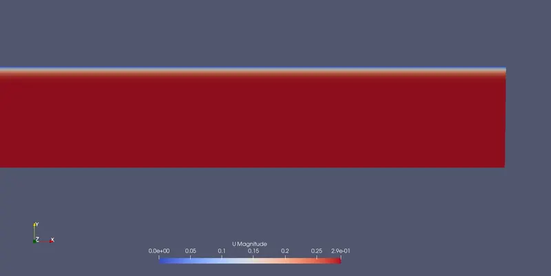
Velocity Contour plot for Hydrodynamic entrance region
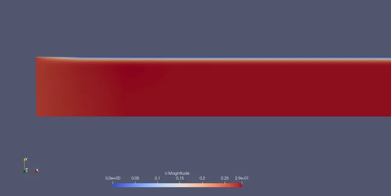
Velocity Contour plot for fully developed flow region
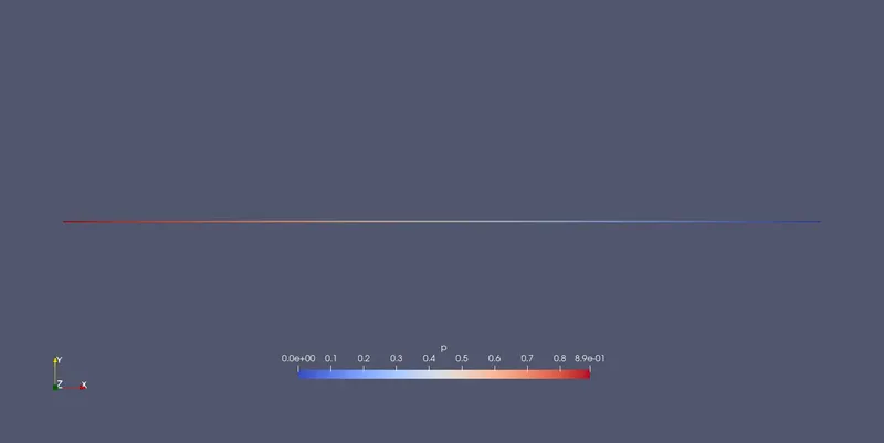
Pressure contour plot for the entire length of the pipe
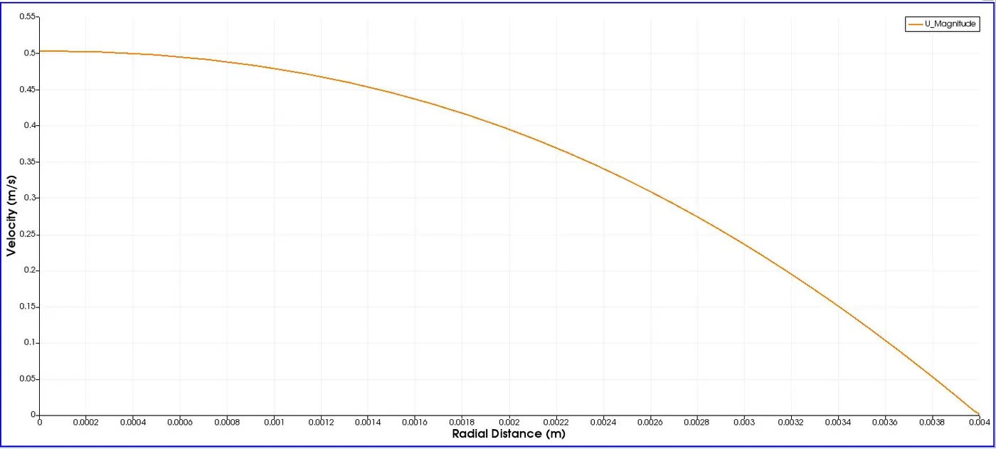
Velocity plot at any point in the hydrodynamic entrance region (say at x = 0.55 m)
Velocity plot at any point in the fully developed flow region (say at x = 1.3 m)
Pressure drop plot for the fully developed flow region (between x = 1.1 m to x = 1.5 m)
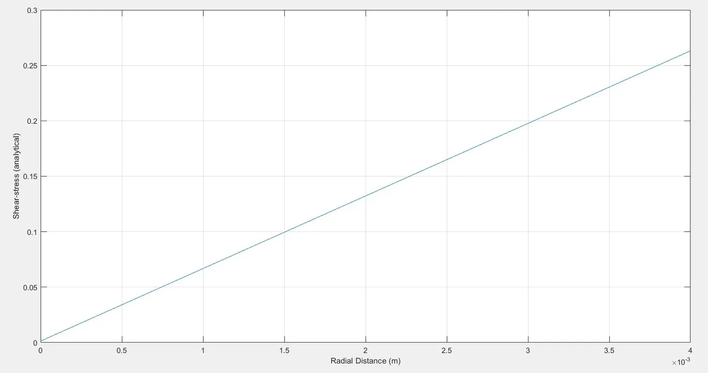
Shear stress plot using analytical solution (`tau = mu(du)/(dy)`)
Shear stress plot using numerical solution
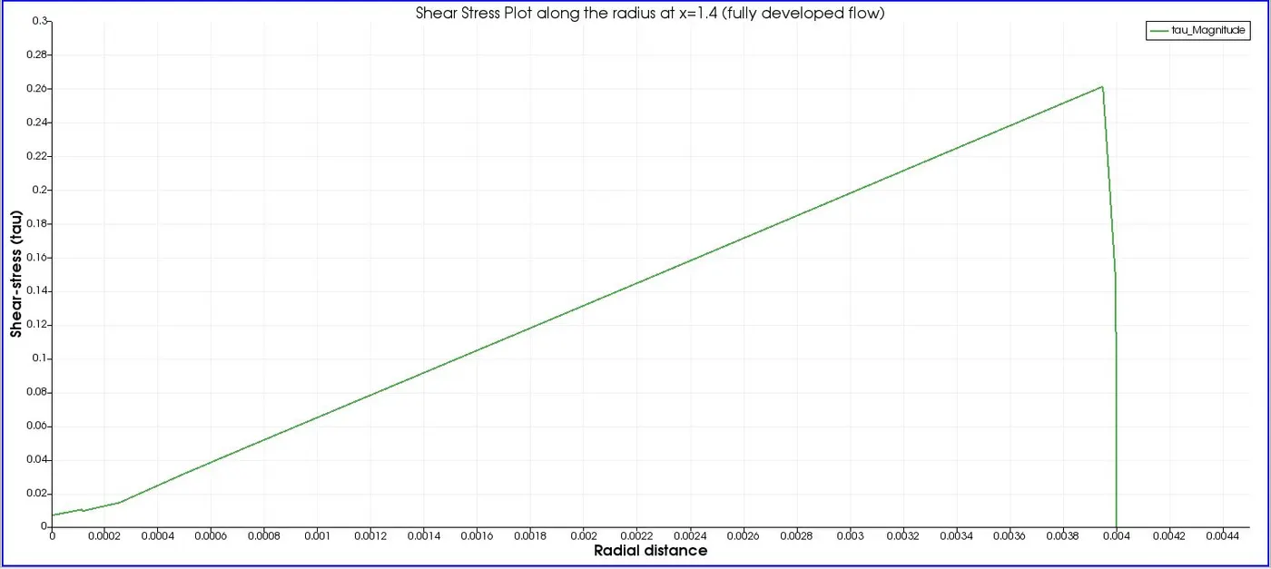
Comparison of analytical and numerical results
| Analytical solution | Numerical solution | Error(%) | |
| Max. velocity (m/s) | 0.5274 | 0.53 | 0.49 |
| Kinematic Pressure (m2/s2) | 0.0529 | 0.0532 | 0.56 |
| Shear stress (N/m2) | 0.260 | 0.261 | 0.38 |
CONCLUSION
- All the necessary contour and xy plots have been plotted for velocity, pressure and shear stress and also the numerical results are validated against the analytical results.
- From the velocity plots, we observe that, for the hydrodynamic entrance region the velocity profile changes, but as the flow reaches to fully developed region, the velocity profile remains constant which is analogous to the Haigen-Poiseuille statement.
- The pressure difference is maximum at the inlet of the pipe, whereas it approaches 0 at the outlet of the pipe.
- Shear stress is maximum at the pipe wall, but it reduces in the radially inward direction towards the centre.