Challenge

Week 11 - Simulation of Flow through a pipe in OpenFoam

SShruti Jadhav10 Oct 2022

CFD MATLAB

Simulate an axi-symmetric flow by applying the wedge boundary condition. The flow is laminar and flows through a constant cross-section pipe at an inlet Reynold's number of 2100. You can do a transient or steady state simulation and you will validate your results with the Hagen- Poiseuille's equations for the fully developed flow.
Objective- To simulate an axi-symmetric flow by applying the wedge boundary condition.
To consider a laminar flow throughout a constant symmetric flow by applying the wedge boundary condition.
To perform a transient or steady state simulation with the Hagen- Poiseuille's equations for the fully developed flow.
Write a matlab code to automate the generation of blockMeshDict file. The code should take inputs like pipe length, diameter, wedge angle, etc and output a fully functional blockMeshDict file.

The flow in which flow variables i.e, velocity and pressure , do not vary with the angular coordinate θ is known a axi-symmetric flow.
The wedge boundary condition is used in computational fluid dynamics to define an axisymmetric situation
The smooth and streamline flows are called laminar flow.

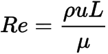
Reynolds number -

where, Re =Reynolds number

= Density of the fluid

= Flow speed

L = length

= Dynamic viscosity of the fluid.

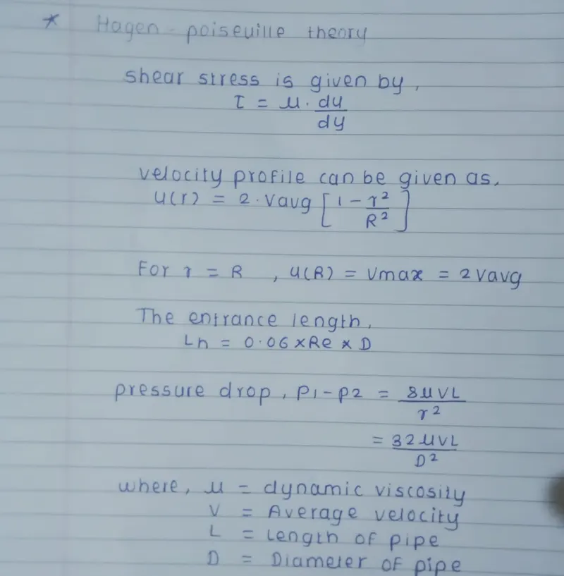
The Hagen-Poiseuille equation describes the parabolic velocity profile of frictional, laminar pipe flows of incompressible Newtonian fluids.
Flows are basically caused by pressure differences that push fluid from places of higher pressure to places of lower pressure .
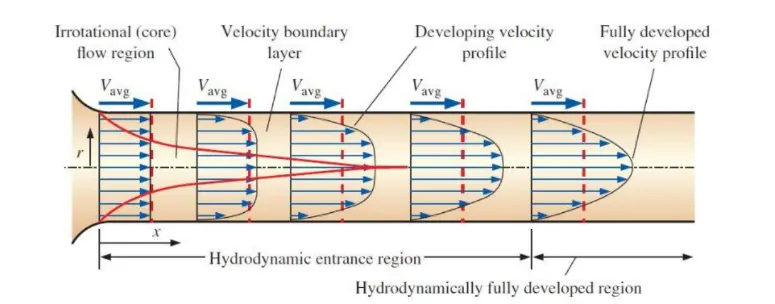
The length of the hydrodynamic inlet describes the formation of a velocity profile caused by viscous forces propagating from the pipe wall.

Formula- shear stress

where, F = Applied force

A= Cross sectional area

For flow through a circular pipe
Re is less than equal to 2300 , then the flow is laminar.
Re is less than equal to 4000 , then the flow is transition.
Re is greater than equal to 4000 , then the flow is turbulent.
Boundary Layer Theory:

Consider a fluid entering a circular pipe with uniform velocity and no slip.

The fluid velocity in the middle section must increase to keep the mass flow through the pipe constant, resulting in a velocity gradient.

The hydrodynamic inlet region is the area from the inlet to the point at which the velocity profile is fully developed, and its length is the hydrodynamic inlet length.
Hagen- Poiseuille's law - The Hagen- Poiseuille's law gives the pressure drop in an incompressible and newtonian fluid in laminar flow flowing through a long cylindrical pipe of constant cross section.
Assumption- The fluid is incompressible and newtonian.

Matlab coding and script for blockMeshDict file

clear all
close all
clc

% Defining Input Values
% Laminar flow
  Re=2100;

% Wedge angle
  theta=2;  

% Diameter of pipe
  D = 0.04; 

% Radius of pipe
  r = D/2

% Hydrodynamic entry length L
 L=0.06*Re*D;

% Assumed characteristic length
 L_c=L+0.3;

% Dynamic viscosity of air
 mu = 1.81e-5

% Density of air
 rho = 1.204

% Kinematic viscosity
  nu=mu/rho 

% calculating average velocity
  v_avg=(mu*Re)/(rho*D)

% Calculating maximum velocity at the centerline of pipe
  v_max=2*v_avg

% Pressure drop for the laminar flow
  delta_p=(32*mu*v_avg*L)/D^2

R=linspace(0,r,400); 
for i=1:length(R)

    tau(i)=2*mu*v_max*(abs(R(i)))/r^2;

end

for j=1: length(R)

    vel_p(j)=2*v_avg*(1-(abs(R(j))^2/r^2));
end

figure(1)
plot(R,tau)
ylabel('Shear stress')
xlabel('Radial length')
 
figure(2)
plot(R,vel_p)
ylabel('Velocity')
xlabel('Radial length')



% Writing the blockMeshDict file

fileid = fopen('blockMeshDict','w');

fprintf(fileid,'This is a test file for blockMesh\n')
fprintf(fileid,'This is my second line\t\tdata\n');
fprintf(fileid,'The Reynolds number is  %f for this simulation',Re);

fprintf(fileid,'\n \t\t(%f\t\t%f\t\t%f)', 0, 0, 0)
fprintf(fileid,'\n \t\t(%f\t\t%f\t\t%f)', r*sind(theta/2), r*cosd(theta/2),0)
fprintf(fileid,'\n \t\t(%f\t\t%f\t\t%f)', -r*sind(theta/2), r*cosd(theta/2),0)
fprintf(fileid,'\n \t\t(%f\t\t%f\t\t%f)', 0, 0, L)
fprintf(fileid,'\n \t\t(%f\t\t%f\t\t%f)', r*sind(theta/2), r*cosd(theta/2),L)
fprintf(fileid,'\n \t\t(%f\t\t%f\t\t%f)', -r*sind(theta/2), r*cosd(theta/2),L)


%blocks
fprintf(fileid,'%s \n','blocks')
fprintf(fileid,'%s \n','(')
fprintf(fileid,'\t hex(0 3 4 1 0 3 5 2) (%d %d %d) simpleGrading (%d %d %d)\n', 200,20,1,1,0.1,1)
fprintf(fileid,'%s \n',');')

%edges
fprintf(fileid,'\n %s \n','edges')
fprintf(fileid,'%s \n','(')
fprintf(fileid,'\t arc 1 2 (%d %d %d) \n',0,r,0)
fprintf(fileid,'\t arc 1 2 (%d %d %d) \n',L,r,0)
fprintf(fileid,'\n %s',');')

%boundary
fprintf(fileid,'\n %s \n','boundary')
fprintf(fileid,'%s \n','(')
fprintf(fileid,'\n %s \n','axis')
fprintf(fileid,'{ \n \t type empty; \n')
fprintf(fileid,'\t faces \n( \n')
fprintf(fileid,'\t (%d %d %d %d) \n',0,3,3,0)
fprintf(fileid,'\t ) ; \n }\n')

%wall
fprintf(fileid,'\n %s \n','wall')
fprintf(fileid,'%s \n','{')
fprintf(fileid,'\t type wall; \n')
fprintf(fileid,'\t faces \n ( \n')
fprintf(fileid,'\t (%d %d %d %d) \n',1,4,5,2)
fprintf(fileid,'\t ) ; \n }\n')

%inlet
fprintf(fileid,'\n %s \n','inlet')
fprintf(fileid,'%s \n','{')

fprintf(fileid,'\t type patch; \n')
fprintf(fileid,'\t faces \n ( \n')
fprintf(fileid,'\t (%d %d %d %d) \n',0,1,2,0)
fprintf(fileid,'\t ) ; \n }\n')

%outlet
fprintf(fileid,'\n %s \n','outlet')
fprintf(fileid,'%s \n','{')
fprintf(fileid,'\t type patch; \n')
fprintf(fileid,'\t faces \n ( \n')
fprintf(fileid,'\t (%d %d %d %d) \n',3,5,4,3)
fprintf(fileid,'\t ); \n }\n')

%front 
fprintf(fileid,'\n\t front \n { \n')
fprintf(fileid,'\t type wedge ; \n')
fprintf(fileid,'\t faces \n ( \n')   
fprintf(fileid,'\t (%d %d %d %d) \n',0,3,4,1)
fprintf(fileid,'\t ) ; \n \t }\n')

%back
fprintf(fileid,'\n\t back \n { \n')
fprintf(fileid,'\t type wedge ; \n')
fprintf(fileid,'\t faces \n ( \n')   
fprintf(fileid,'\t (%d %d %d %d) \n',0,2,5,3)
fprintf(fileid,'\t ) ; \n \t }\n')

fprintf(fileid,');')
fclose(fileid)

Stepwise Explaination of the code-
Assign initial Hagen-Pousville flow rates values.
% Laminar flow

Re=2100;

% Wedge angle

theta=2;

Calculation of properties such as dynamic viscosity, average speed, maximum speed, inlet length.
Change in pressure value is calculated with the hagen-pousville formula.
Linspace command is used to store the array function.
Calculate the shear stress and velocity profile using a for loop.
Plotting values to obtain an analytical solution.
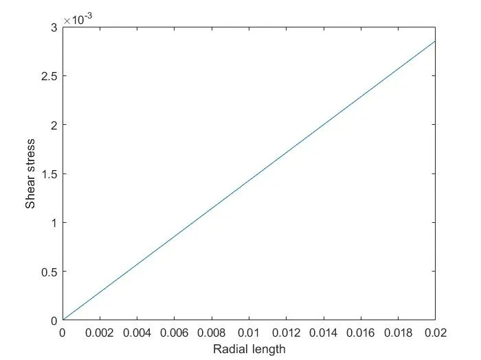
Shear stress vs radial length and velocity vs radial length graph are plotted.
Create a BlockMeshDict file using the write function:
Assign vertices at all points of the wedge. (v1, v2, v3, v4, v5)
Create a controlDict file using the write function
Drafting the blockMeshDict file using the write function in MATLAB.
The drafting should be done with a similar pattern as the blockMeshDict file used in openFoam.
Writing the vertices of the wedge .
Assigning edges, walls, borders, entry, exit, front and back of blocks.
Create a pressure and velocity file using the write function and make changes accordingly.
Using paraview mesh are created and graphs are plotted.
Flow simulation procedure:

A. To select the solver and copy the folder

1. Open terminal command in ubuntu.

2. open tutorials, code: tut

3. Open the incompressible folder and select icofoam, then cavity. (code: icoFoam)

4. Copy the cavity folder to the startup folder. using code: 'cp -r pipr/$FOAM_RUN'

5. Type the run command to open the run folder.

6. Open the pipe. (code: cd pipe)

( Also copy and paste the blockMeshDict file created by MATLAB into the system folder)

7. Open the system file.

8. Run the blockMeshDict code file. (code: blockMesh)
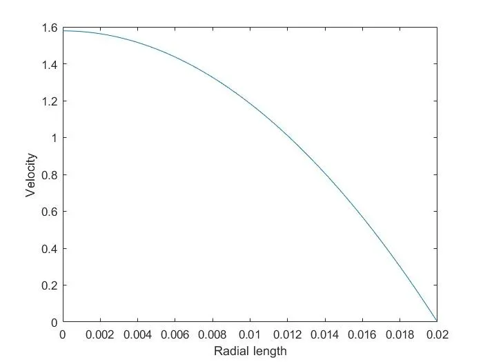
Results- plot- Velocity vs Radial Length

Shear stress vs radial length

BlockMeshDict

/*--------------------------------*- C++ -*----------------------------------*\
  =========                 |
  \\      /  F ield         | OpenFOAM: The Open Source CFD Toolbox
   \\    /   O peration     | Website:  https://openfoam.org
    \\  /    A nd           | Version:  10
     \\/     M anipulation  |
\*---------------------------------------------------------------------------*/
FoamFile
{
    format      ascii;
    class       dictionary;
    object      blockMeshDict;
}
// * * * * * * * * * * * * * * * * * * * * * * * * * * * * * * * * * * * * * //

convertToMeters 1;

vertices
(
		(0.000000		0.000000		0.000000)
 		(0.000349		0.019997		0.000000)
 		(-0.000349		0.019997		0.000000)
 		(0.000000		0.000000		5.040000)
 		(0.000349		0.019997		5.040000)
 		(-0.000349		0.019997		5.040000)
);

blocks 
( 
	 hex (0 3 4 1 0 3 5 2) (200 20 1) simpleGrading (1 1 1)
); 

 edges 
( 
	 arc 1 2 (0 2.000000e-02 0) 
	 arc 4 5 (5.040000e+00 2.000000e-02 0) 

 );
 boundary 
( 

 axis 
{ 
 	 type empty; 
	 faces 
( 
	 (0 3 3 0) 
	 ) ; 
 }

 wall 
{ 
	 type wall; 
	 faces 
 ( 
	 (1 4 5 2) 
	 ) ; 
 }

 inlet 
{ 
	 type patch; 
	 faces 
 ( 
	 (0 1 2 0) 
	 ) ; 
 }

 outlet 
{ 
	 type patch; 
	 faces 
 ( 
	 (3 5 4 3) 
	 ); 
 }
front 
 { 
	 type wedge ; 
	 faces 
 ( 
	 (0 3 4 1) 
	 ) ; 
 	 }
back 
 { 
	 type wedge ; 
	 faces 
 ( 
	 (0 2 5 3) 
	 ) ; 
 	 }
);

controlDict

/*--------------------------------*- C++ -*----------------------------------*\
  =========                 |
  \\      /  F ield         | OpenFOAM: The Open Source CFD Toolbox
   \\    /   O peration     | Website:  https://openfoam.org
    \\  /    A nd           | Version:  10
     \\/     M anipulation  |
\*---------------------------------------------------------------------------*/
FoamFile
{
    format      ascii;
    class       dictionary;
    location    "system";
    object      controlDict;
}
// * * * * * * * * * * * * * * * * * * * * * * * * * * * * * * * * * * * * * //

application     icoFoam;

startFrom       startTime;

startTime       0;

stopAt          endTime;

endTime         0.04;

deltaT          0.005;

writeControl    timeStep;

writeInterval   20;

purgeWrite      0;

writeFormat     ascii;

writePrecision  6;

writeCompression off;

timeFormat      general;

timePrecision   6;

runTimeModifiable true;


// ************************************************************************* //

Pressure-

/*--------------------------------*- C++ -*----------------------------------*\
  =========                 |
  \\      /  F ield         | OpenFOAM: The Open Source CFD Toolbox
   \\    /   O peration     | Website:  https://openfoam.org
    \\  /    A nd           | Version:  10
     \\/     M anipulation  |
\*---------------------------------------------------------------------------*/
FoamFile
{
    format      ascii;
    class       volScalarField;
    object      p;
}
// * * * * * * * * * * * * * * * * * * * * * * * * * * * * * * * * * * * * * //

dimensions      [0 2 -2 0 0 0 0];

internalField   uniform 0;

boundaryField
{
    inlet
    {
        type            zeroGradient;
    }

    outlet

    axis
    {
        type            empty;
    }

    {
        type            fixedValue;
        value           uniform 0;
    }

    wall
    {
        type            zeroGradient;
    }
    
    front
    {
        type            wedge;
    }
   
    Back
    {
        type             wedge;
    }

// ************************************************************************* //

Velocity

/*--------------------------------*- C++ -*----------------------------------*\
  =========                 |
  \\      /  F ield         | OpenFOAM: The Open Source CFD Toolbox
   \\    /   O peration     | Website:  https://openfoam.org
    \\  /    A nd           | Version:  10
     \\/     M anipulation  |
\*---------------------------------------------------------------------------*/
FoamFile
{
    format      ascii;
    class       volVectorField;
    object      U;
}
// * * * * * * * * * * * * * * * * * * * * * * * * * * * * * * * * * * * * * //

dimensions      [0 1 -1 0 0 0 0];

internalField   uniform (0 0 0.020);

boundaryField
{
    inlet
    {
        type            fixedValue;
        value           uniform (0 0 0.020);
    }

   outlet
    {

       type             zeroGradient;
    }

    axis
    {
        type            empty;
    }
    
    wall

    {
        type            noSlip;
    }

    front

    {
        type            wedge;
    }

    Back
    {
        type            wedge;
    }
}

// ************************************************************************* //

Open paraview:

1. Change directory to block_test

2. Run code: checkMesh

3. Run code:icoFoam

4. Run code: paraFoam

5. In paraview click apply.
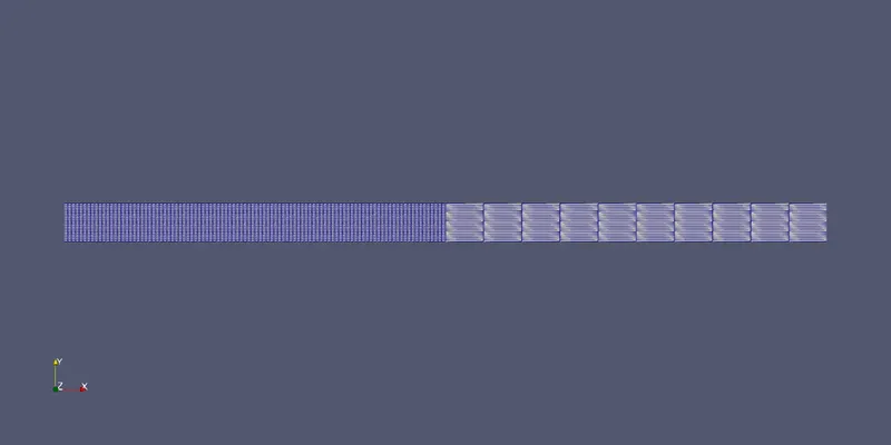
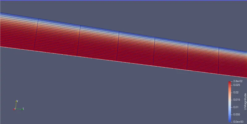
Resulted geometry created by blockMeshDict file - Mesh

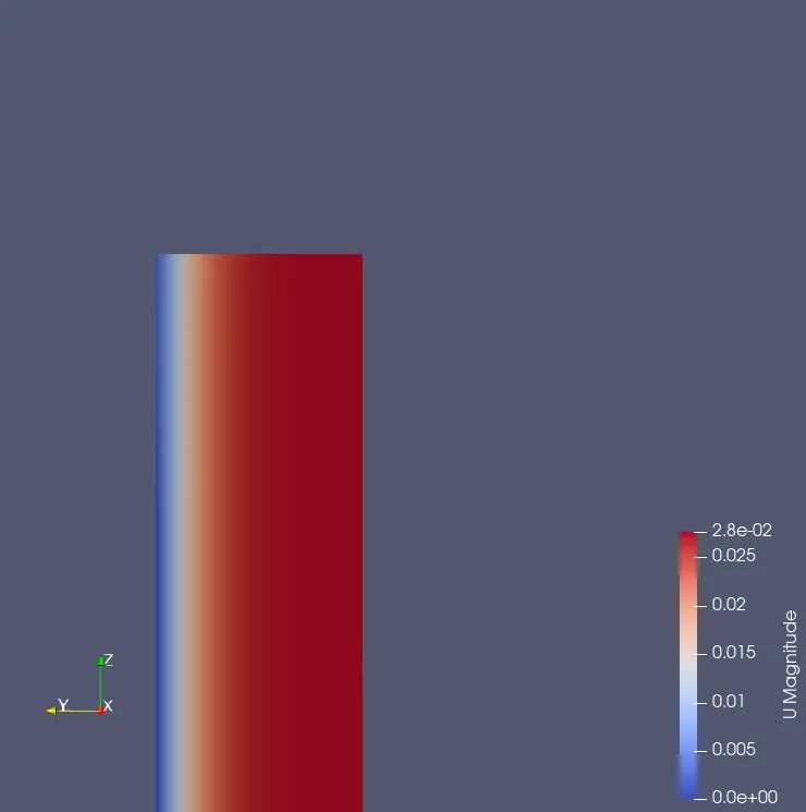
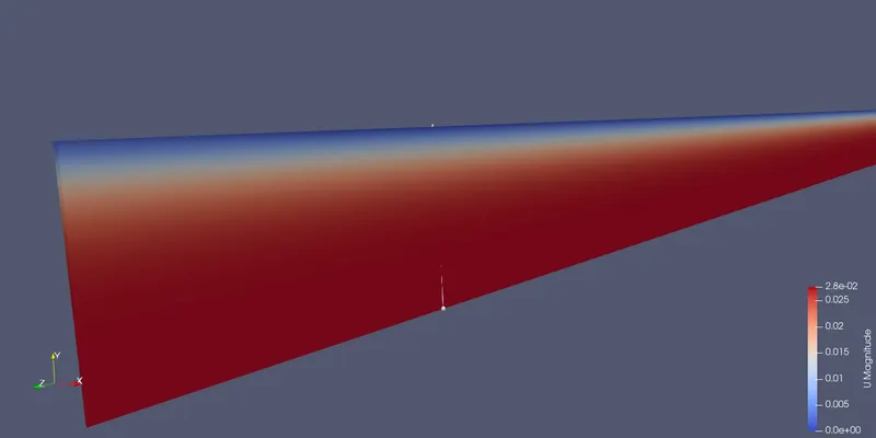
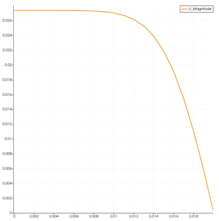
Velocity plot at distance x= 2.385

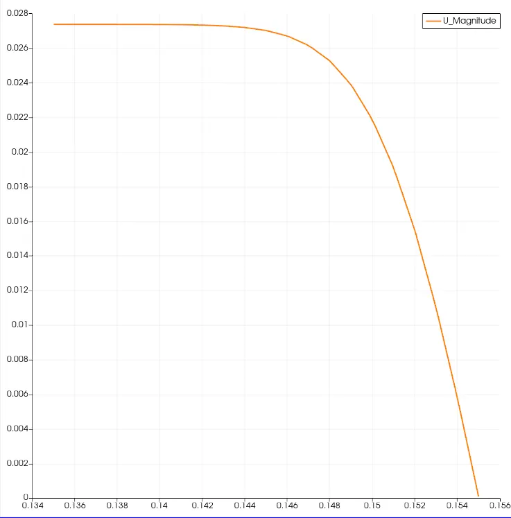
Velocity plot at a distance x = 1.22

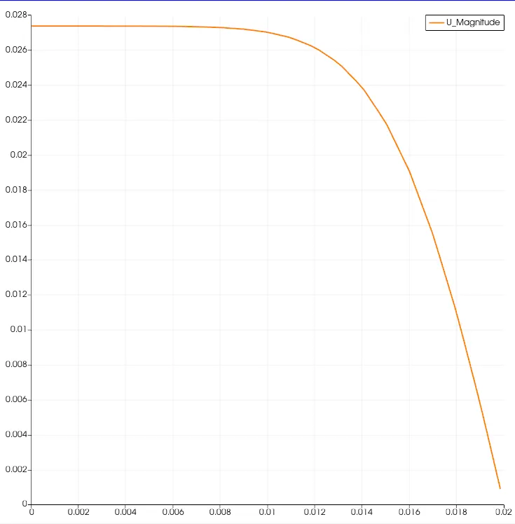
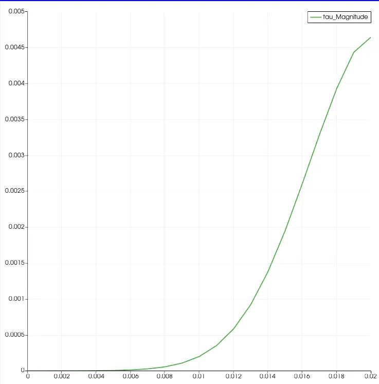
Shear stress plot for wedge angle 2.

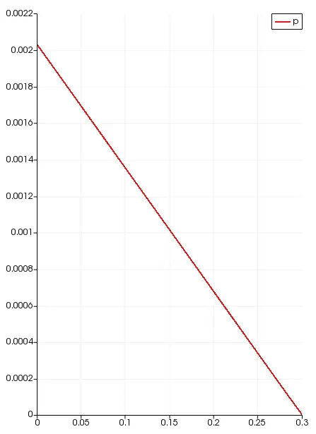
Pressure drop plot

Conclusion-
The velocity profile is plotted at varying distances from the inlet of the pipe.
By increasing the radial length shear stress increases.
The shear stress is zero at the center of the pipe and increases linearly towards the wall, the graph obtained from openfoam is close to the analytical result.
The maximum velocity and pressure drop value is achieved for fully developed flow.
Pressure drop and length of pipe is directly proportional.
The hydrodynamic length is obtained at 2.52 units where the velocity profile is fully developed.
The velocity profile gradually increases from inlet to outlet. After the flow is fully developed, it remains constant.
The analytical velocity profile and the velocity obtained in openfoam agree very well, where the velocity is maximum in the center and decreases parabolically towards the wall.

Week 11 - Simulation of Flow through a pipe in OpenFoam

Ship work like this
in your own course.

Talk to a career counsellor

Ship work like thisin your own course.

Talk to a career counsellor

Ship work like this
in your own course.