Week 11 - Simulation of Flow through a pipe in OpenFoam

Aim :  to simulate flow through pipe using openfoam

objective:

•  to simulate an axi-symmetric flow by applying the wedge boundary condition.explain about how to extract the vertices from the wedge boundary.
• to validate your results with the Hagen- Poiseuille's equations for the fully developed flow.
• to write code in Matlab to automate the generation of blockMeshDict file. The code should take inputs like pipe length, diameter, wedge angle, etc and output a fully functional blockMeshDict file. 

Expected Results are

1. Validate Hydro-dynamic length with the numerical result
2. Validate the fully developed flow velocity profile with its analytical profile
3. Validate maximum velocity and pressured drop for fully developed flow
4. Post-process Shear stress and validate wall shear stress for fully developed flow

Hints are given to follow the calculations for the 

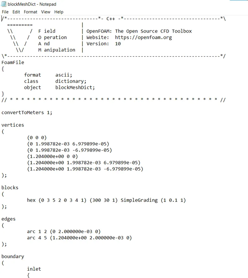
1. create a wedge from a hex block by collapsing its bottom face (by merging both sets of adjacent vertices)
2. Wedge angle should be less than 5 degrees
3. You can assume the pipe diameter.
4. The flow is laminar and flows through a constant cross-section pipe at an inlet Reynold's number of 2100. You can do a transient or steady state simulation.

MATLAB programming :

clear all 
close all 
clc

%input & assumption values

%reynolds number
Re=2100;

%diameter of the pipe
D=0.004;

%entry length of the pipe
L=0.06*Re*D;

%total length of the pipe
L_p=L+0.7;

%radius of the pipe 
r=D/2;

%angle of wedge(angle must be less than 5)
theta=4;

%density
rho=997;

%dynamic viscosity
mu=0.89e-3;

%creating analytical velocity formula
%hagen poisuilleis equation
V_avg=(Re*mu)/(rho*D);
y=linspace(0,r,20);
u=2*V_avg*(1-(y.^2/r^2));

figure(1)
plot(y,u)
ylabel('velocity')
xlabel('radial distance')
legend('radial distance varies')

V_max =2*V_avg;

%calculate shear stress
dy = y(2)-y(1);
tau=(2*mu*V_max.*y)./(r^2)

figure(2)
plot(y,tau)
ylabel('shear stress')
xlabel('radial distance')
legend('shear stress development')




deltap=(32*mu*L_p*V_avg)/(D^2);

header1='/*--------------------------------*- C++ -*----------------------------------*\';
header2='  =========                 |';
header3='  \\      /  F ield         | OpenFOAM: The Open Source CFD Toolbox';
header4='   \\    /   O peration     | Website:  https://openfoam.org';
header5='    \\  /    A nd           | Version:  10';
header6='     \\/     M anipulation  |';
header7='\*---------------------------------------------------------------------------*/';

f1=fopen("blockMeshDict","w");
fprintf(f1,'%s\n',header1);
fprintf(f1,'%s\n',header2);
fprintf(f1,'%s\n',header3);
fprintf(f1,'%s\n',header4);
fprintf(f1,'%s\n',header5);
fprintf(f1,'%s\n',header6);
fprintf(f1,'%s\n',header7);

fprintf(f1,'%s\n','FoamFile');
fprintf(f1,'%s\n','{');
fprintf(f1,'\tformat     ascii;\n');
fprintf(f1,'\tclass      dictionary;\n');
fprintf(f1,'\tobject     blockMeshDict\n');
fprintf(f1,'%s\n','}');
header8='// * * * * * * * * * * * * * * * * * * * * * * * * * * * * * * * * * * * * * //';
fprintf(f1,'%s\n\n',header8);

fprintf(f1,'%s\n\n','convertToMeters 1;');
fprintf(f1,'%s\n','vertices;');
fprintf(f1,'%s\n','(');
fprintf(f1,'\t (%d %d %d)\n',0,0,0);
fprintf(f1,'\t (%d %d %d)\n',0,r*cosd(theta/2),r*sind(theta/2));
fprintf(f1,'\t (%d %d %d)\n',0,r*cosd(theta/2),-r*sind(theta/2));
fprintf(f1,'\t (%d %d %d)\n',L_p,0,0);
fprintf(f1,'\t (%d %d %d)\n',L_p,r*cosd(theta/2),r*sind(theta/2));
fprintf(f1,'\t (%d %d %d)\n',L_p,r*cosd(theta/2),-r*sind(theta/2));
fprintf(f1,'%s\n\n',');');

fprintf(f1,'%s\n','blocks');
fprintf(f1,'%s\n','(');
fprintf(f1,'\t hex (0 3 5 2 0 3 4 1) (%d %d %d)\n',300,30,1);
fprintf(f1,' SimpleGrading (1 0.1 1)\n');
fprintf(f1,'%s\n\n',');');

fprintf(f1,'%s\n','edges');
fprintf(f1,'%s\n','(');
fprintf(f1,'\t arc %d %d (%d %d %d)\n',1,2,0,r,0);
fprintf(f1,'\t arc %d %d (%d %d %d)\n',4,5,L_p,r,0);
fprintf(f1,'%s\n\n',');');

fprintf(f1,'%s\n','boundary');
fprintf(f1,'%s\n','(');
fprintf(f1,'\t inlet \n');
fprintf(f1,'\t {\n');
fprintf(f1,'\t\t type patch;\n');
fprintf(f1,'\t\t faces\n');
fprintf(f1,'\t\t (\n');
fprintf(f1,'\t\t\t (0 1 2 0)\n');
fprintf(f1,'\t\t );\n');
fprintf(f1,'\t }\n');

fprintf(f1,'%s\n','(');
fprintf(f1,'\t outlet \n');
fprintf(f1,'\t {\n');
fprintf(f1,'\t\t type patch;\n');
fprintf(f1,'\t\t faces\n');
fprintf(f1,'\t\t (\n');
fprintf(f1,'\t\t\t (3 5 4 3)\n');
fprintf(f1,'\t\t );\n');
fprintf(f1,'\t }\n');

fprintf(f1,'%s\n','(');
fprintf(f1,'\t top \n');
fprintf(f1,'\t {\n');
fprintf(f1,'\t\t type wall;\n');
fprintf(f1,'\t\t faces\n');
fprintf(f1,'\t\t (\n');
fprintf(f1,'\t\t\t (1 4 5 2)\n');
fprintf(f1,'\t\t );\n');
fprintf(f1,'\t }\n');

fprintf(f1,'%s\n','(');
fprintf(f1,'\t front \n');
fprintf(f1,'\t {\n');
fprintf(f1,'\t\t type wedge;\n');
fprintf(f1,'\t\t faces\n');
fprintf(f1,'\t\t (\n');
fprintf(f1,'\t\t\t (0 3 4 1)\n');
fprintf(f1,'\t\t );\n');
fprintf(f1,'\t }\n');

fprintf(f1,'%s\n','(');
fprintf(f1,'\t back \n');
fprintf(f1,'\t {\n');
fprintf(f1,'\t\t type wedge;\n');
fprintf(f1,'\t\t faces\n');
fprintf(f1,'\t\t (\n');
fprintf(f1,'\t\t\t (0 2 5 3)\n');
fprintf(f1,'\t\t );\n');
fprintf(f1,'\t }\n');

fprintf(f1,'%s\n','(');
fprintf(f1,'\t axis \n');
fprintf(f1,'\t {\n');
fprintf(f1,'\t\t type empty;\n');
fprintf(f1,'\t\t faces\n');
fprintf(f1,'\t\t (\n');
fprintf(f1,'\t\t\t (0 3 3 0)\n');
fprintf(f1,'\t\t );\n');
fprintf(f1,'\t }\n');
fprintf(f1,'%s\n\n',');');

fprintf(f1,'%s\n','mergePatchPairs');
fprintf(f1,'%s\n','(');
fprintf(f1,'%s\n',');');
header9='// * * * * * * * * * * * * * * * * * * * * * * * * * * * * * * * * * * * * * //';
fprintf(f1,'%s\n',header9);

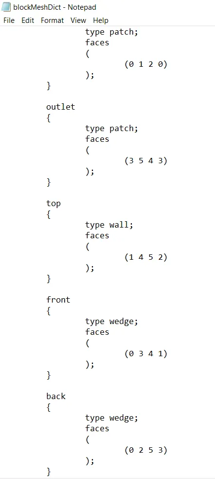
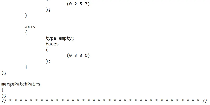
BlockmeshDict :

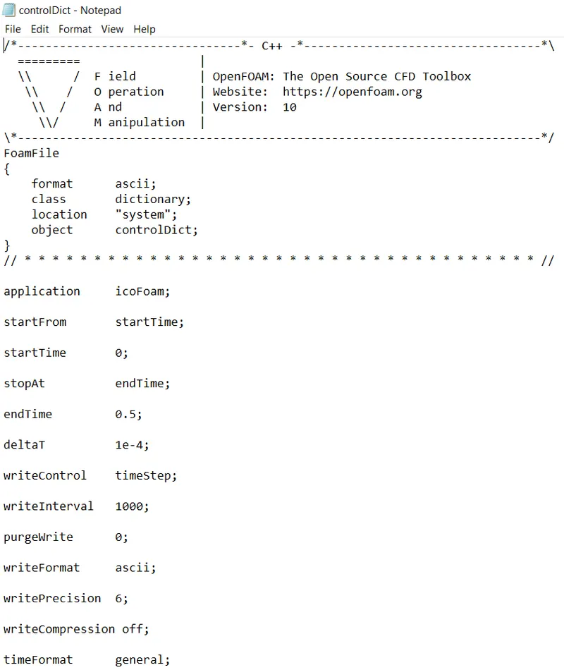
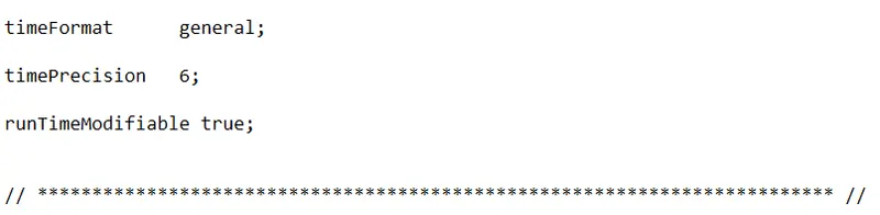
Controldict file :

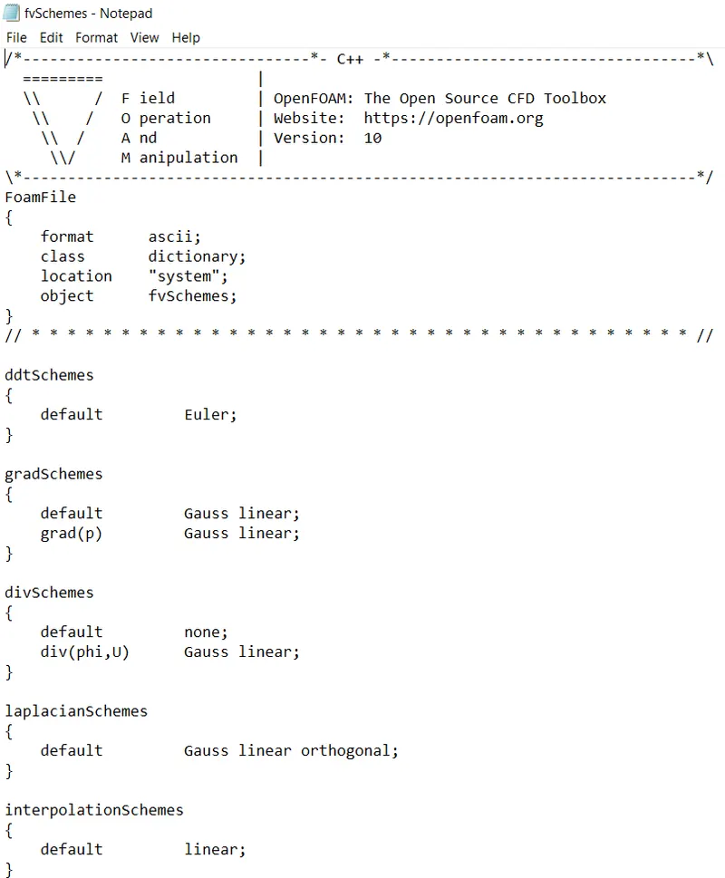
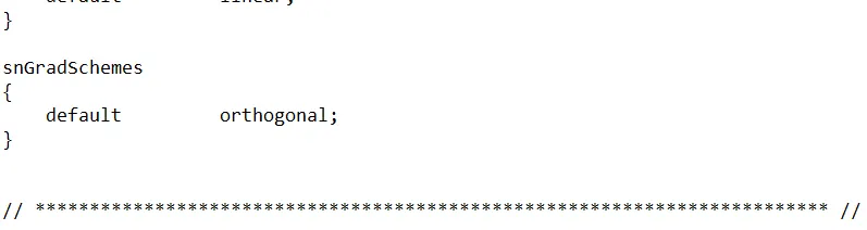
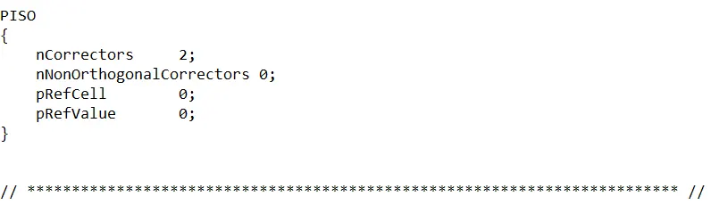
fv schemes :

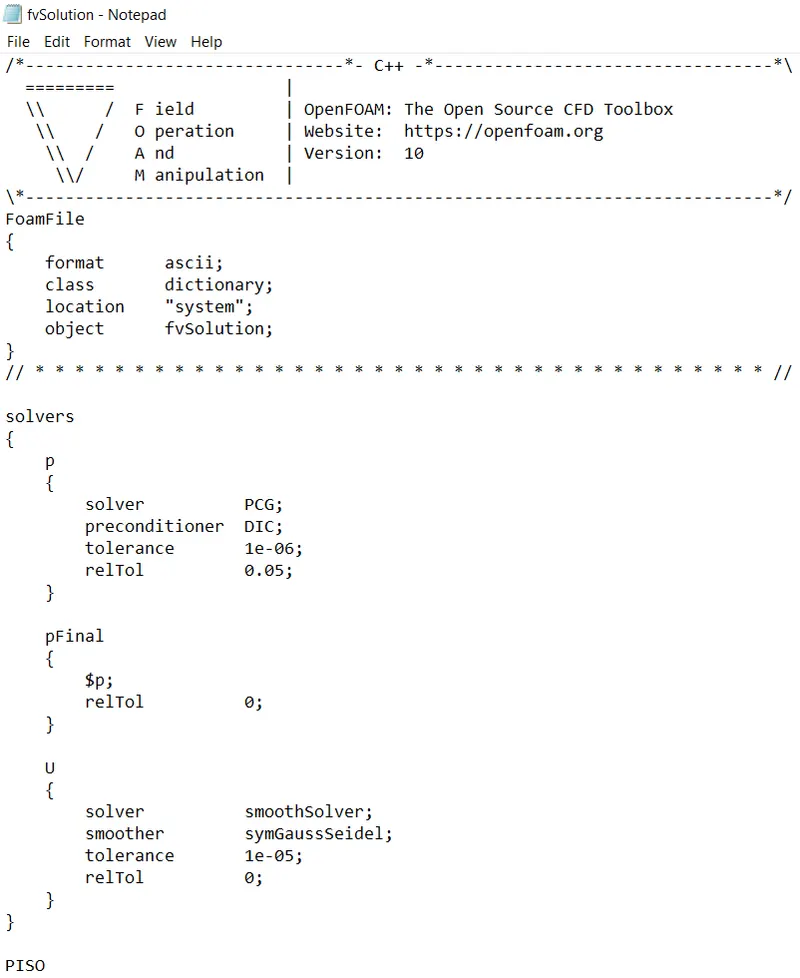
fv Solutions :

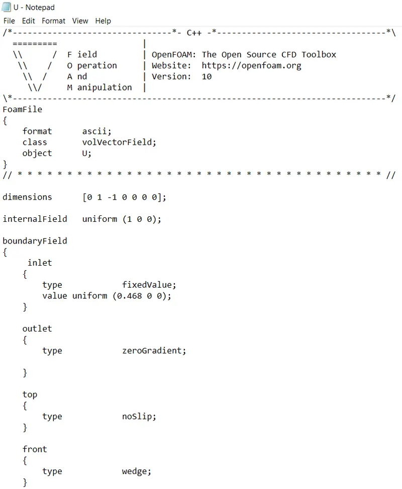
velocity profile :

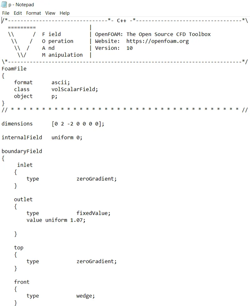
pressure profile :

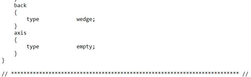
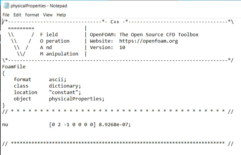
physical properties :

 MATLAB program explantation :

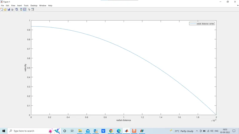
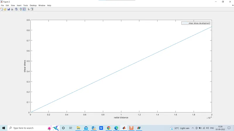
1)initially define all the given values and after find out the maximum velocity and the total length of pipe and shear stress calculations in a therictical way.and then plot a figure between radial distance and the velocity & radial distance and the  shear stress

2)create a block mechdict file by using the inbuild commands in matlab as per the boundary conditions and the given conditions.

paraview :

1)after creating the files we will have to check wheather the blockmesh dict file is correct or not by using blockmesh command in ubuntu terminal and then check wheather the mesh is correct or not by using checkmesh command and use icofoam solver and then directly go to the paraview to visualise the result.

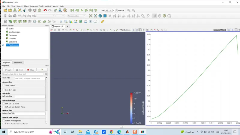
2)view the block and see wheather the block is create as per the given conditions or not.then click on surface with edges option and then select velocity profile and the oressure profile one by one then set the axis we want to visualize the result.

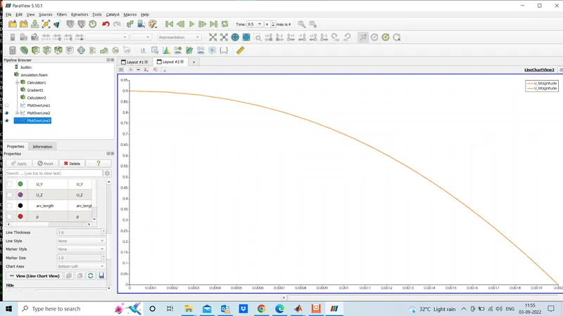
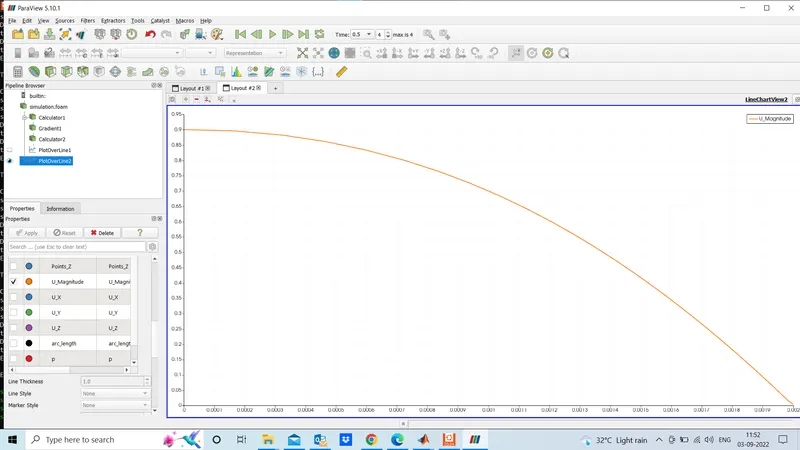
3)by selecting plot over line command we will be able to we can select the velocity profile and see how the velocity changes over the period fluid moves 

4)velocity is gradually decreasing the at the wall and gradually increasing at the centre of the block so that it can maintain ythe mass flow rate through out the domain from the inlet to the outlet.velocity profile varies till it becomes 0 at the wall because of the resistance due to fluid and solid interaction.where the velocity profile increases half is called as hydrodynamically half developed region.and fully developed region is called as hydrodynamically fully developed region.

shear stress :

1)shear stress is gradually increase at wall section since wall regions resist the flow inside the boundary.se will be creating a shear stress profile in paraview to visualise how tit chsnges across the domain until the velocity reaches to zero at no slip condition.then we will compare both the analytical and numerical values and compare both and if the values are very close to each then the values are considered to be a valid and we can proceed with it.

 

conclusion :

if we compare both the theoritical and the numerical application results the shear stress values are equalt to 0.85 and also the velocity from both the analytical and the numerical value is equal to 0.95m/s so the results we have got here is valid.