Week 11 - Simulation of Flow through a pipe in OpenFoam
Objective:
Simulation of flow through a pipe
- Finding out the velocity, pressure and shear stress profile for a fully developed flow
- To validate the results with analytical values
- To create a wedge of wedge angle not less than 5 degrees , and simulate the flow through it.
Hagen poiseuilles flow:
The Hagen poiseuilles flow describes the relationship between pressure , fluidic resistemce and flow rate analogous to voltage , resistence and current respectively in Ohms law for electric circuits.
Assumption :
- The flow is steady
- The flow is laminar
Consider stationary , laminar flow in apipe with viscosity `mu` , flow rate `Q` and average velocity `U`,pipe length `L`, radius `r` . The pressure drop `dP=(-8*mu*L)/(r^2)*U`
The shear stress distribution is given by:
`tau=(-(delP)/(delx))*(r/2)`
By analysing the above equation, it can be inferred that, the shear stress varies linearlly with the radial distance from the centre of the pipe. It is minimum at the centre of the pipe, that is zero. And at the walls, it is maximum.
The velocity distribution along the pipe is given by:
`u=(1/(4*mu))*((-delP)/(delx))*(R^2-r^2)`
The above equation is the local velocity profile. This gives the velocity profile at any radial location in the pipe. At the centre, r=0, and at the walls, r=R. So the velocity is maximum at the centre and minimum or zero at the walls. The maximum velocity is given as :
`u_max=2*u_mean`
Hydrodynamic entrance length:
The hydrodynamic entrance length is defined some what as the duct length required to achieve a duct section maximum velocity of 99% of the corresponding fully developed magnitude when enterring flow is uniform.For laminar flow through pipes, The hydrodynamic entrance length is given by
`L_h=0.05*Re*D`
Here, `Re,D` are the reynolds number of the flow and the Diameter of the pipe.
A matlab code is written to automate the generation of blockMeshDict file.
The idea of the simulation is that, the pipe is cut into a wedge, for an angle theta. the value of theta is kept below 5 degrees.
Boundary conditions:
1) Inlet and outlet is given type patch.
2) front and back is given type wedge.
3) Axis is given type empty.
Control parameters:
The start time of the simulation is 0 seconds and the end time is 1 seconds. The time step can be manipuilated . Since an explicit formulation, the Courant number must be within limits. the dt is given a value 0.0001.
Matlab code for automating the blockMeshDict file:
clear all
close all
clc
%flow parameters

Re =2100;%reynolds number
D=0.004;%diameter of the pipe
r=D/2;%radius of the pipe
l=0.06*Re*D;%hydrodynamic entrance length
l_p=l+0.7;%length of the pipe
theta=5;%wedge angle
mu=0.89e-03;%dynamic viscosity
rho=997;%density of fluid
v_avg=(Re*mu)/(rho*D);%mean velocity
v_max=2*v_avg;%maximum velocity
del_p=(8*mu*l_p*v_avg)/(r^2);%pressure drop
kin_p=(del_p)/(rho);%kinematic pressure drop
%Writing the blockMeshDict file
f1=fopen('blockMeshdict','w');
%defining the vertioces
fprintf(f1, 'vertices\n');
fprintf(f1, '(\n');
fprintf(f1, '\t (%d %d %d)\n',0,0,0);
fprintf(f1, '\t (%d %d %d)\n',0,r*cosd(theta/2),r*sind(theta/2));
fprintf(f1, '\t (%d %d %d)\n',0,r*cosd(theta/2),-r*sind(theta/2));
fprintf(f1, '\t (%d %d %d)\n',l,0,0);
fprintf(f1, '\t (%d %d %d)\n',l,r*cosd(theta/2),r*sind(theta/2));
fprintf(f1, '\t (%d %d %d)\n',l,r*cosd(theta/2),-r*sind(theta/2));
fprintf(f1, ');\n\n');
fprintf(f1, 'blocks\n');
fprintf(f1, '(\n');
fprintf(f1, '\t hex(0 3 5 2 0 3 4 1)(%d %d %d)',300,30,1);
fprintf(f1, 'SimpleGrading (1 0.1 1)\n\n');
fprintf(f1, ');\n\n');

fprintf(f1, 'edges\n');
fprintf(f1, '(\n');
fprintf(f1, '\t arc %d %d (%d%d%d)\n',1,2,0,r,0);
fprintf(f1, '\t arc %d %d(%d %d %d)\n',4,5,l_p,r,0);
fprintf(f1, ');\n\n');

%boundary conditions
fprintf(f1, 'boundary\n');
fprintf(f1, '(\n');
fprintf(f1, '\t inlet \n');
fprintf(f1, '\t {\n');
fprintf(f1, '\t {\n');
fprintf(f1, '\t\t type patch;\n');
fprintf(f1, '\t\t faces \n');
fprintf(f1, '\t\t\t (0 1 2 0)\n');
fprintf(f1, '\t\t); \n');
fprintf(f1, '\t }\n');

fprintf(f1, '\t outlet\n');
fprintf(f1, '\t {\n');
fprintf(f1, '\t\t type patch ;\n');
fprintf(f1, '\t\t faces\n');
fprintf(f1, '\t\t (\n');
fprintf(f1, '\t\t\t (3 5 4 3)\n');
fprintf(f1, '\t\t); \n');
fprintf(f1, '\t }\n');

fprintf(f1, '\t top\n');
fprintf(f1, '\t {\n');
fprintf(f1, '\t\t type wall;\n');
fprintf(f1, '\t\t faces\n');
fprintf(f1, '\t\t (\n');
fprintf(f1, '\t\t\t (1 4 5 2)\n');
fprintf(f1, '\t\t);\n');
fprintf(f1, '\t\t); \n');
fprintf(f1, '\t} \n');

fprintf(f1, '\t front\n');
fprintf(f1, '\t{\n');
fprintf(f1, '\t\t type wedge;\n');
fprintf(f1, '\t\t faces\n');
fprintf(f1, '\t\t (\n');
fprintf(f1, '\t\t\t (0 3 4 1) \n');
fprintf(f1, '\t\t );\n');
fprintf(f1, '\ }\n');


fprintf(f1, '\t back\n');
fprintf(f1, '\t{\n');
fprintf(f1, '\t\t type wedge ;\n');
fprintf(f1, '\t\t faces\n');
fprintf(f1, '\t\t (\n');
fprintf(f1, '\t\t\t (0 2 5 3)\n');
fprintf(f1, '\t\t);\n');
fprintf(f1, '\t }\n');


fprintf(f1, '\t axis\n');
fprintf(f1, '\t{\n');
fprintf(f1, '\t\t type empty;\n');
fprintf(f1, '\t\t faces\n');
fprintf(f1, '\t\t (\n');
fprintf(f1, '\t\t\t (0 3 3 0)\n');
fprintf(f1, '\t}\n');
fprintf(f1, '); \n\n');
BlockmeshDict file:
/*--------------------------------*- C++ -*----------------------------------*\
  =========                 |
  \\      /  F ield         | OpenFOAM: The Open Source CFD Toolbox
   \\    /   O peration     | Website:  https://openfoam.org
    \\  /    A nd           | Version:  8
     \\/     M anipulation  |
\*---------------------------------------------------------------------------*/
FoamFile
{
    version     2.0;
    format      ascii;
    class       dictionary;
    object      blockMeshDict;
}
// * * * * * * * * * * * * * * * * * * * * * * * * * * * * * * * * * * * * * //

convertToMeters 1;
vertices
(
	 (0 0 0)
	 (0 1.998096e-03 8.723877e-05)
	 (0 1.998096e-03 -8.723877e-05)
	 (5.040000e-01 0 0)
	 (5.040000e-01 1.998096e-03 8.723877e-05)
	 (5.040000e-01 1.998096e-03 -8.723877e-05)
);

blocks
(
	 hex (0 3 5 2 0 3 4 1) (300 30 1) SimpleGrading (1 0.1 1)

);

edges
(
	 arc 1 2 (0 2.000000e-03 0)
	 arc 4 5 (1.204000e+00 2.000000e-03 0)
);

boundary
(
	 inlet
	 {
		 type patch;
		 faces
		 (
			 (0 1 2 0)
		 );
	 }
	 outlet
	 {
		 type patch ;
		 faces
		 (
			 (3 5 4 3)
		 );
	 }
	 top
	 {
		 type wall;
		 faces
		 (
			 (1 4 5 2)
		 );

	}
	front
	{
		 type wedge;
		 faces
		 (
			 (0 3 4 1)
		 );
        }
	back
	{
		 type wedge ;
		 faces
		 (
			 (0 2 5 3)
		 );
	 }
	 axis
	 {
		 type empty;
		 faces
		 (
			 (0 3 3 0)
	         );
	 }
);


mergePatchPairs
(
);

// ************************************************************************* //
controlDict file::
/*--------------------------------*- C++ -*----------------------------------*\
  =========                 |
  \\      /  F ield         | OpenFOAM: The Open Source CFD Toolbox
   \\    /   O peration     | Website:  https://openfoam.org
    \\  /    A nd           | Version:  8
     \\/     M anipulation  |
\*---------------------------------------------------------------------------*/
FoamFile
{
    version     2.0;
    format      ascii;
    class       dictionary;
    location    "system";
    object      controlDict;
}
// * * * * * * * * * * * * * * * * * * * * * * * * * * * * * * * * * * * * * //

application     icoFoam;

startFrom       startTime;

startTime       0;

stopAt          endTime;

endTime         1;

deltaT          0.0001;

writeControl    timeStep;

writeInterval   20;

purgeWrite      0;

writeFormat     ascii;

writePrecision  6;

writeCompression off;

timeFormat      general;

timePrecision   6;

runTimeModifiable true;


// ************************************************************************* //
pressure file:
/*--------------------------------*- C++ -*----------------------------------*\
  =========                 |
  \\      /  F ield         | OpenFOAM: The Open Source CFD Toolbox
   \\    /   O peration     | Website:  https://openfoam.org
    \\  /    A nd           | Version:  8
     \\/     M anipulation  |
\*---------------------------------------------------------------------------*/
FoamFile
{
    version     2.0;
    format      ascii;
    class       volScalarField;
    object      p;
}
// * * * * * * * * * * * * * * * * * * * * * * * * * * * * * * * * * * * * * //

dimensions      [0 2 -2 0 0 0 0];

internalField   uniform 0;

boundaryField
{
    inlet
    {
        type            zeroGradient;
    }

    outlet
    {
        type            fixedValue;
        value uniform 1.0073;
    }

    axis
    {
        type            empty;
    }
    top
    {
        type            zeroGradient;
    }
    front
    {
        type            wedge;
    }
    back
    {
        type            wedge;
    }

}

// ************************************************************************* //
Velocity file:
/*--------------------------------*- C++ -*----------------------------------*\
  =========                 |
  \\      /  F ield         | OpenFOAM: The Open Source CFD Toolbox
   \\    /   O peration     | Website:  https://openfoam.org
    \\  /    A nd           | Version:  8
     \\/     M anipulation  |
\*---------------------------------------------------------------------------*/
FoamFile
{
    version     2.0;
    format      ascii;
    class       volVectorField;
    object      U;
}
// * * * * * * * * * * * * * * * * * * * * * * * * * * * * * * * * * * * * * //

dimensions      [0 1 -1 0 0 0 0];

internalField   uniform (0.4686 0 0);

boundaryField
{
    inlet
    {
        type            fixedValue;
        value           uniform (0.4686 0 0);
    }

    outlet
    {
        type            zeroGradient;
    }

    axis
    {
        type            empty;
    }
    top
    {
        type            fixedValue;
        value uniform (0 0 0);
    }
    front
    {
        type            wedge;
    }
    back
    {
        type            wedge;
    }
}

// ************************************************************************* //
By running the command, blockMesh, the blocks are created. We can check the mesh, if it is fine , by running the command, checkMesh. To run the simulation, icoFoam command is usde.
The simulation took nearly 655 seconds to complete. Here a explicit formulation is solved. The minimum and maximum Courant number is: 0.028 and 0.09. That is well between the limits. In the simulation process, if floating point exception error is encountered, The dt or the time step value should be reduced further. As changing the dx value is bit complicated.
Post-processing:
- Grid generation:
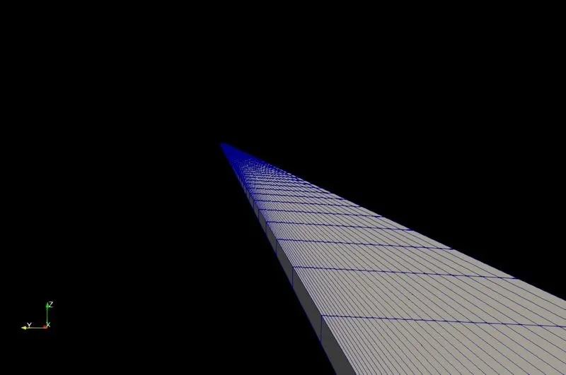
It is bit challenging to orient the wedge in the correct manner in paraview. Still , its a good one to visualize the surface with edges.
- Velocity contour:
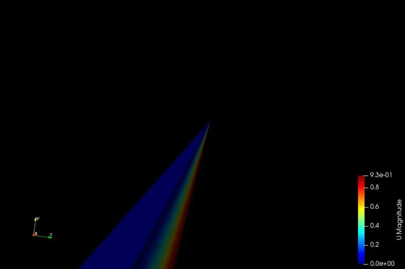
The maximum velocity is 0.93 m/s. the wedge section is perfectly visualized from the contour.
- pressure contour
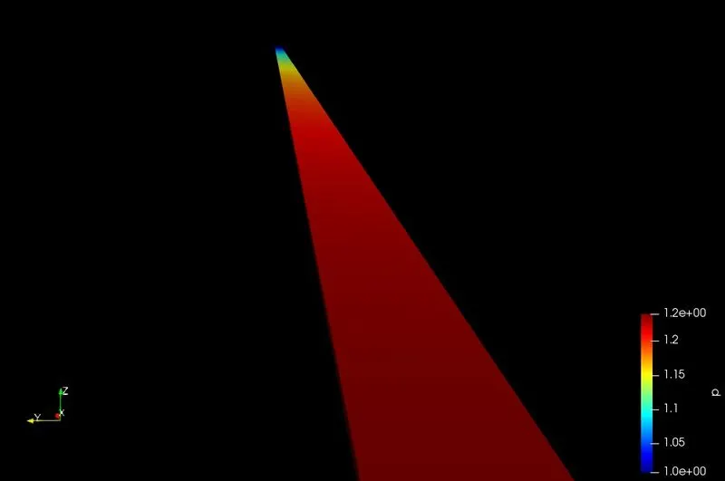
The maximum pressure is 1.2 pas.
Velocity profile at differnt sections using line probe.
In paraview, we can plot, the velocity at different location using the plot over line feature. To visualize the velocity proifile along the y-direction, at different x locations. from the formula of the velocity profile it can be attributed that the velocity varies radially along the pipe. After the hydrodynamic entrance length, the full velocity profile is obtained.
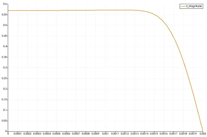
the above plot is the velocioty profile, when the line probe is taken at a point, inside the hydrodynamic entrance length. The plot is just at the entrance of the flow to the pipe.
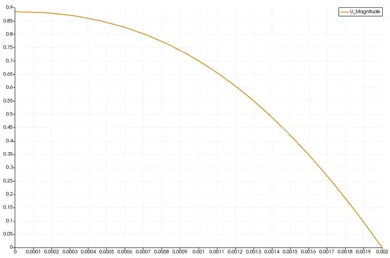
This is the velocity profile obtained, when the line probve is set at a location outside the hydrodynamic entrance length.
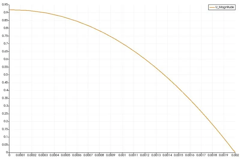
This is at one end of the pipe.
Shear stress plot:
This is obtained in paraview by slight manipualtion.
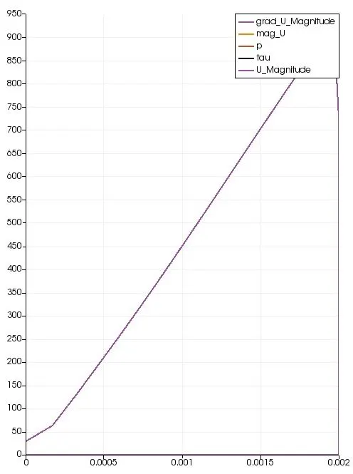
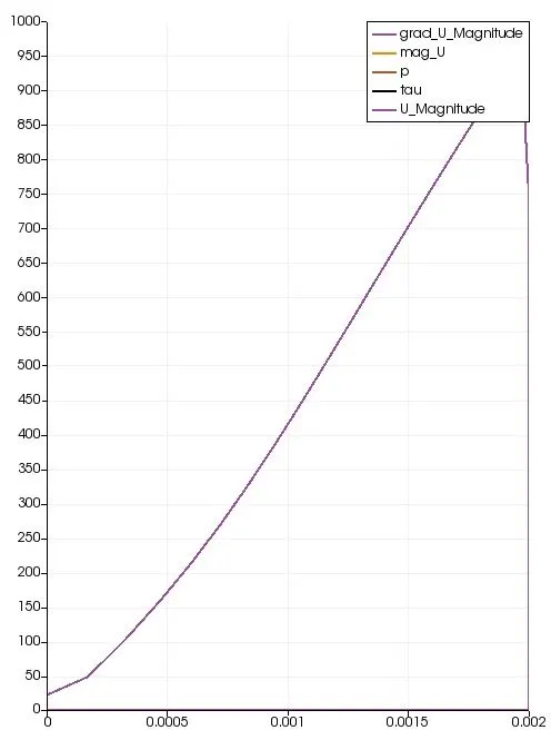
First of all , using a calculator, the magnitude of velocity(mag(U) ) is calculated. This is plotted. Now enabling the gradient of unstructuired data, The shear stress is calcuklated using the calculator. The formula for the shear stress is `tau=mu*(du)/(dy)`
here, we first calculated the magnitude of velcity vector acroos the domain. Then by multiplying the dynamic viscosity with this value, we obtain the shear stress.
To plot the shear stress across the domain, we use plot over line:
- Pressure plot:
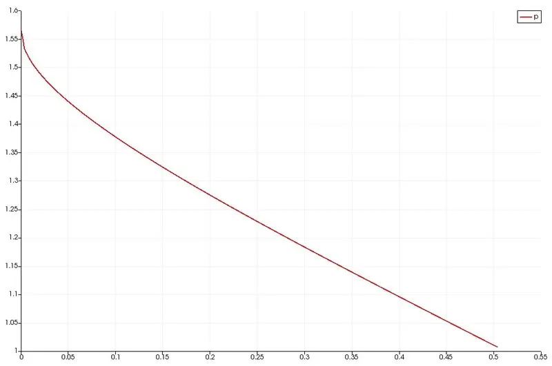
The pressure variation is linear .
the shear stress is minimu at the centre and maximum at tthe walls.
Validation of results :
| Simulation data | Analytical results | Error | |
| maximum velocity | 0.93 m/s | 0.94 m/s | 1.06 % |
| mean velocity | 0.465 m/s | 0.47 m/s | 1.03% |
| Maximum wall shear stress | 900 N/m^2 | ||
| Hydrodynamic entrance length | 0.4 m | 0.42 m |
Conclusion:
- A flow through a pipe is simulated.
- The maximum velocity and and the hydrodynamic entrance length value is validated with analytical results.