Simulation of Flow through a pipe in OpenFOAM
Simulation of Flow through a pipe in OpenFoam
AIM:
1. To simulate an axis-symmetric flow by applying the wedge boundary condition. The flow is laminar and flows through a constant cross-section pipe at an inlet Reynold's number of 2100.
2. To validate the simulation results with the Hagen- Poiseuille's equations for the fully developed flow.
3. Also to write code in Matlab to automate the generation of blockMeshDict file. The code will take inputs like pipe length, diameter, wedge angle, etc, and output a fully functional blockMeshDict file.
THEORY:
Introduction to Internal Flow:
Liquid or gas flow through pipes or ducts is commonly used in heating and cooling applications and fluid distribution networks. The fluid in such applications is usually forced to flow by a fan or pump through a flow section. The terms pipe, duct, and conduit are usually used interchangeably for flow sections. In general, flow sections of the circular cross-section are referred to as pipes (especially when the fluid is a liquid) and flow sections of the non-circular cross-section as ducts (especially when the fluid is a gas). Small diameter pipes are usually referred to as tubes.
The fluid velocity in a pipe changes from zero at the wall because of the no-slip condition to a maximum at the pipe center. In fluid flow, it is convenient to work with an average velocity Vavg, which remains constant in incompressible flow when the cross-sectional area of the pipe is constant(refer to image 1.1)
Also, the friction between the fluid particles in a pipe does cause a slight rise in fluid temperature as a result of the mechanical energy being converted to sensible thermal energy. But this temperature rise due to frictional heating is usually too small to warrant any consideration in calculations and thus is disregarded.
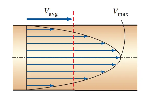
Image 1.1 Fully developed laminar pipe flow.
Laminar Flow and Turbulent Flow:
Laminar flow or streamline flow in pipes (or tubes) occurs when a fluid flows in parallel layers, with no disruption between the layers. At low velocities, the fluid tends to flow without lateral mixing, and adjacent layers slide past one another like playing cards. There are no cross-currents perpendicular to the direction of flow, nor eddies or swirls of fluids. In laminar flow, the motion of the particles of the fluid is very orderly with all particles moving in straight lines parallel to the pipe walls.
Turbulent flow is a flow regime characterized by chaotic property changes. This includes rapid variation of pressure and flows velocity in space and time. In contrast to laminar flow, the fluid no longer travels in layers, and mixing across the tube is highly efficient. Flows at Reynolds numbers larger than 4000 are typically (but not necessarily) turbulent, while those at low Reynolds numbers below 2300 usually remain laminar. Flow in the range of Reynolds numbers 2300 to 4000 and known as transition.
Reynolds Number:
The transition from laminar to turbulent flow depends on the geometry, surface roughness, flow velocity, surface temperature, and type of fluid, among other things. After exhaustive experiments in the 1880s, Osborne Reynolds discovered that the flow regime depends mainly on the ratio of inertial forces to viscous forces in the fluid. This ratio is called the Reynolds number and is expressed for internal flow in a circular pipe as
`R_e = text(Inertia Force)/text(Viscous Force) = (V_(avg)D)/nu=(rhoV_(avg)D)/mu`
where `V_(avg)` = average flow velocity `(m//s)`, `D =` characteristic length of the geometry (diameter in this case, in `m`), and `nu = mu/rho =` kinematic viscosity of the fluid `(m^2//s)`.
The Entrance Length or Hydrodynamic Length:
Consider a fluid entering a circular pipe at a uniform velocity. Because of the no-slip condition, the fluid particles in the layer in contact with the wall of the pipe come to a complete stop. This layer also causes the fluid particles in the adjacent layers to slow down gradually as a result of friction. To make up for this velocity reduction, the velocity of the fluid at the midsection of the pipe has to increase to keep the mass flow rate through the pipe constant. As a result, a velocity gradient develops along the pipe.
The region of the flow in which the effects of the viscous shearing forces caused by fluid viscosity are felt is called the velocity boundary layer or just the boundary layer. The hypothetical boundary surface divides the flow in a pipe into two regions: the boundary layer region, in which the viscous effects and the velocity changes are significant, and the irrotational (core) flow region, in which the frictional effects are negligible and the velocity remains essentially constant in the radial direction.
The thickness of this boundary layer increases in the flow direction until the boundary layer reaches the pipe center and thus fills the entire pipe, as shown in Image 1.2, and the velocity becomes fully developed a little farther downstream. The region from the pipe inlet to the point at which the velocity profile is fully developed is called the hydrodynamic entrance region, and the length of this region is called the hydrodynamic entry length `L_h`. Flow in the entrance region is called hydrodynamically developing flow since this is the region where the velocity profile develops. The region beyond the entrance region in which the velocity profile is fully developed and remains unchanged is called the hydrodynamically fully developed region. The flow is said to be fully developed when the normalized temperature profile remains unchanged as well.
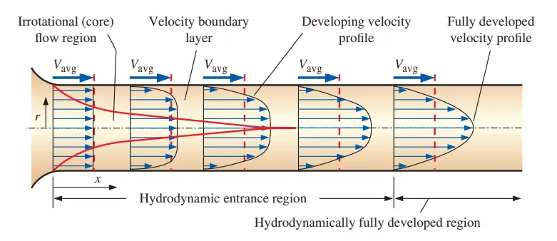
Image 1.2 The development of the velocity boundary layer in a pipe.
Entry Length:
The hydrodynamic entry length(refer the image 1.3) is usually taken to be the distance from the pipe entrance to where the wall shear stress (and thus the friction factor) reaches within about 2 percent of the fully developed value. In laminar flow, the nondimensional hydrodynamic entry length is given approximately as
`L_(h, text(laminar))/D approx 0.05R_e`
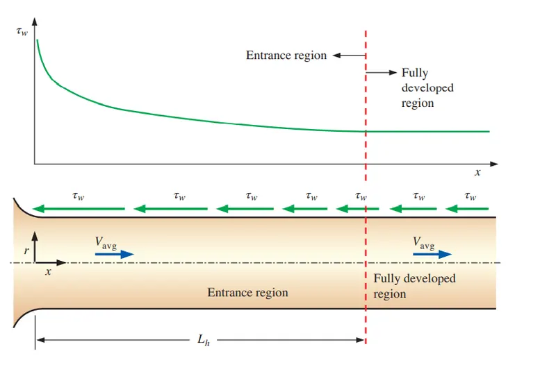
Image 1.3 The variation of wall shear stress in the flow direction for flow in a pipe from the entrance region into the fully developed region.
Laminar Flow Through Pipe:
Consider the steady, laminar, incompressible flow of fluid with constant properties in the fully developed region of a straight circular pipe. The momentum equation obtained by applying a momentum balance to a differential volume element, and also the velocity profile is obtained by solving it. Then it is used to obtain a relation for the friction factor. An important aspect of the analysis here is that it is one of the few available for viscous flow.
In fully developed laminar flow, each fluid particle moves at a constant axial velocity along a streamline and the velocity profile u(r) remains unchanged in the flow direction. There is no motion in the radial direction, and thus the velocity component in the direction normal to the pipe axis is everywhere zero. There is no acceleration since the flow is steady and fully developed.
The velocity profile is fully developed laminar flow in a pipe is parabolic with a maximum at the centerline and a minimum (zero) at the pipe wall and is given by the equation as a function of radial distance from the center.
`u(r) = 2V_(avg)(1-r^2/R^2)`
The pressure drop due to viscous effects over the length of the pipe is shown below(refer the image 1.4)
`triangleP = P_1 - P_2 = (8muLV_(avg))/R^2`
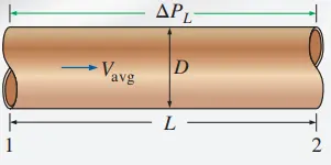
Image 1.4 The pressure drop due to viscous effects
PROCEDURE:
For this simulation of Flow-Through axis-symmetric all the above formulae are used to simulate the flow. Since the model is axis-symmetric only a small wedge is modeled such that this wedge is a symmetric part of the Cylinder(refer to the below image).
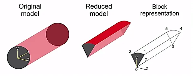
Image 2.1 Reduced Model of the Axis Symmetric Model.
In te above-reduced figure of the axis-symmetric model, the block consists of 6 vertices namely 0,1,2,3,4,5 where the face 012 is Inlet, 345 is the outlet, 1254 is the wall of the cylinder and the 0253 and 0341 is the wedge patch.
Developing the blockMeshDict file:
To develop the blockMeshDict file first the wedge dimension are calculated. The wedge dimensions are calculated using the given details.
Given Details:
Reynold's Number, `R_e` = 2100.
Assuming the value of Diameter,
Diameter, d = 0.01m.(r = 0.005m)
Fluid = Water at 303K.
Kinamatic Viscosity at 303K = `0.801xx10^-6 m^2//s`
Density of the Water at 303K =` 995kg//m^3`
Dynamic Viscosity at 303K = 0.000797Pa s
Wedge Angle = `3^o`(less than `5^o`)
The theoritical hydrodynamic length
`L_(h,text(laminar)) = 0.05xx2100xx0.01`
`L_(h,text(laminar)) = 1.05m`
Since the Hydrodynamic Length is 1.05m, let the length of the pipe be 1.2m so that the fully developed flow can be seen after 1.05m.
From the Reynolds Number fromula
`2100 = (V xx 1.2)/(0.801xx10^-6`
` V = 0.1682m//s`
Simulation time is the time taken by the fluid to travel the length of the pipe.
Simulation Time = `l/V`sec
`therefore` `t = 7.13`
To see the fully developed flow the simulation is run for more time and hence it is simulated for 10 seconds.
Calculation of Coordinates of the Verticies of the Wedge
[0] = (0,0,0)
[1] = (0,`rcos(alpha/2)`,`rsin(alpha/2)`)
[2] = (0,`rcos(alpha/2)`,`-rsin(alpha/2)`)
[3] = (1.2,0,0)
[4] = (1.2,`rcos(alpha/2)`,`rsin(alpha/2)`)
[5] = (1.2,`rcos(alpha/2)`,`-rsin(alpha/2)`)
The coordinates are calculates from the principles of trigonometry.
Solver for the simulation:
The icoFoam solver in the OpenFOAM tutorials is used for this simulation. In that solver, a slight modification is done for the requirement. The modifications are as follows
Modification 1: Change in blockMeshDict file
The blockMeshDict file is modified as per the model. From the above calculations, the blockMeshDict file is modified as below.
/*--------------------------------*- C++ -*----------------------------------*
| =========                 |                                                 |
| \      /  F ield         | OpenFOAM: The Open Source CFD Toolbox           |
|  \    /   O peration     | Version:  v2012                                 |
|   \  /    A nd           | Website:  www.openfoam.com                      |
|    \/     M anipulation  |                                                 |
*---------------------------------------------------------------------------*/
FoamFile
{
    version     2.0;
    format      ascii;
    class       dictionary;
    object      blockMeshDict;
}
// * * * * * * * * * * * * * * * * * * * * * * * * * * * * * * * * * * * * * //

convertToMeter   0.1;


vertices
(
    (0 0 0)
    (0 0.00499829 0.000130885)
    (0 0.00499829 -0.000130885)
    (1.2 0 0)
    (1.2 0.00499829 0.000130885)
    (1.2 0.00499829 -0.000130885)
);

blocks
(
    hex (0 2 1 0 3 5 4 3) (20 1 100) simpleGrading (0.2 1 1)
);


edges
(
);

boundary
(

    inlet
    {
        type patch;
        faces
        (
            (0 1 2 0)
        );
    }

    outlet
    {
        type patch;
        faces
        (
            (3 4 5 3)
        );
    }

    sideface01
    {
        type wedge;
        faces
        (
            (0 2 5 3)
        );
    }

    sideface02
    {
        type wedge;
        faces
        (
            (0 1 4 3)
        );
    }

    noSlipWalls
    {
    	type wall;
    	faces
    	(
    	     (2 1 4 5)
    	);
    }

    axis
    {
    	type empty;
    	faces
    	(
    	     (0 3 3 0)
    	);
    }
);

mergePatchPairs
(
);

// ************************************************************************* //
In the above code, only single block is created and the simple grading 0.2 is given so that the mesh is finer near the walls. Also, the along the length 100 divisions are made, along the radial distance 20 divisions are made and only 1 division is made along the thickness. Also for all the faces, respective patches are created.
Program to develop the blockMeshDict file:
In the above code, most of the code is text and the coordinates are dependant on the diameter, length, and wedge angle. Therefore the developed program receives the diameter, length, and wedge angle and gives out the blockMeshDict file.
clear all
close all
clc

alpha = input('Wedge Angle:');
l = input('Pipe Length:');
d = input('Pipe Diameter:');

fid = fopen( 'blockMeshDict', 'wt' );
%Inital Comments
fprintf(fid,"/*--------------------------------*- C++ -*----------------------------------*\n");
fprintf(fid,'| =========                 |                                                 |n');
fprintf(fid,"| \\      /  F ield         | OpenFOAM: The Open Source CFD Toolbox           |n");
fprintf(fid,'|  \\    /   O peration     | Version:  v2012                                 |n');
fprintf(fid,'|   \\  /    A nd           | Website:  www.openfoam.com                      |n');
fprintf(fid,'|    \\/     M anipulation  |                                                 |n');
fprintf(fid,"\*---------------------------------------------------------------------------*/ n");
%File Version,Format etc
fprintf(fid,'FoamFilen');
fprintf(fid,'{n');
fprintf(fid,'    version     2.0;n');
fprintf(fid,'    format      ascii;n');
fprintf(fid,'    class       dictionary;n');
fprintf(fid,'    object      blockMeshDict;n');
fprintf(fid,'} n');
fprintf(fid,'// * * * * * * * * * * * * * * * * * * * * * * * * * * * * * * * * * * * * * //n');
%Scale
fprintf(fid,"nconvertToMeter   0.1;nn");

fprintf(fid,"nverticesn");

% Wedge Parameters.
A1 = (d/2)*sind(alpha/2);
OA = (d/2)*cosd(alpha/2);

fprintf(fid,'( n    (0 0 0)n    (0 %d %d)n',OA,A1);
fprintf(fid,'    (0 %d -%d)n    (%d 0 0)n    (%d %d %d)n    (%d %d -%d)n);n', OA,A1,l,l,OA,A1,l,OA,A1 );
%Block
fprintf(fid,'nblocksn');
fprintf(fid,"(n    hex (0 2 1 0 3 5 4 3) (20 1 100) simpleGrading (0.2 1 1)n);nn");
%Edges
fprintf(fid,'nedgesn(n);n');
%Boundary
fprintf(fid,'nboundaryn(n');
%Inlet
fprintf(fid,'n    inletn    {n        type patch;n        facesn');
fprintf(fid,'        (n            (0 1 2 0)n        );n    }n');
%Outlet
fprintf(fid,'n    outletn    {n        type patch;n        facesn');
fprintf(fid,'        (n            (3 4 5 3)n        );n    }n');
%SideFace01
fprintf(fid,'n    sideface01n    {n        type wedge;n        facesn');
fprintf(fid,'        (n            (0 2 5 3)n        );n    }n');
%SideFace02
fprintf(fid,'n    sideface02n    {n        type wedge;n        facesn');
fprintf(fid,'        (n            (0 1 4 3)n        );n    }n');
%noSlipWalls
fprintf(fid,'n    noSlipWallsn    {n    	type wall;n');
fprintf(fid,'    	facesn    	(n    	     (2 1 4 5)n    	);n    }n')

%axis
fprintf(fid,'n    axisn    {n    	type empty;n');
fprintf(fid,'    	facesn    	(n    	     (0 3 3 0)n    	);n    }n);n')

%Mergepairs
fprintf(fid,'nmergePatchPairsn(n);nn');

fprintf(fid,"// ************************************************************************* //n");

fclose(fid);
Modification 2: Changes in the p, U file.
In both files, the patches are to updated and in the U file, the inlet velocity is to be updated.
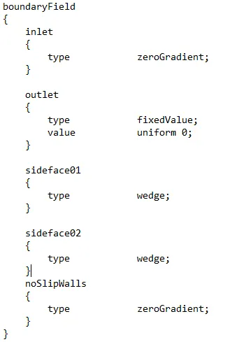
Image 2.2 p file
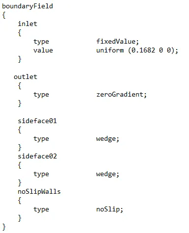
Image 2.3 U file
Modification 3: Changes in the Transport properties file
Updating the Kinematic Viscosity `nu`
nu [0 2 -1 0 0 0 0] 0.801e-6;Modification 4: Changes in controlDict file
In this file, the starting time, end time, and the time step according to the CFL criteria. The CFL number should be less than 1 and is calculates as follows
`CFL number = (Uxxtrianglet)/(trianglex)`
where the `trianglet` = time step size, `trianglex`= minimum element length.
Here the minimum element length is
`trianglex = 1.2/100 = 0.012`
Let `trianglet = 0.01sec`
`CFL number = (0.1682xx0.01)/0.012`
`CFL number = 0.1401`
Since the CFL number is less than 1, the simulation will run without any errors.
About the Solver: icoFoam solver
icoFoam solves the incompressible laminar Navier-Stokes equations using the PISO algorithm. The code is inherently transient, requiring an initial condition (such as zero velocity) and boundary conditions. The icoFOAM code can take mesh non-orthogonality into account with successive non-orthogonality iterations. The number of PISO corrections and non-orthogonality corrections are controlled through user input.
Running the simulation:
To create the polymesh in the OpenFOAM first the run folder is opened and blockMesh code is executed and it ran successfully without any errors. After creating the polymesh icoFoam code is executed to run the simulation. The simulation ran without any errors and took around a minute to run the simulation.
After running the simulation below code is executed as it was running in WSL ubuntu.
touch simulation.foamThis will create a file that is used to view the simulation in the ParaView.
RESULTS:
To view the results, the simulation.foam file is opened in the ParaView. Since the length of the pipe is very large when compared to the radial distance the model looks like a straight line as shown below.
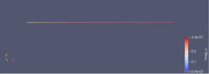
Image 3.1 Results
Plotting the Velocity Profile along the radial distance:
Plot over line command is used to plot the velocity profile.
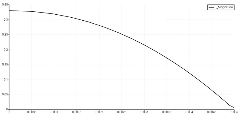
Image 3.2 Velocity profile at distance 1.1m from the inlet.
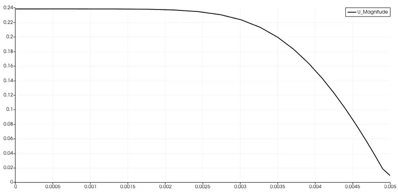
Image 3.3 Velocity profile at distance 0.1m from the inlet.
The region from the pipe inlet to the point at which the velocity profile is fully developed is called the hydrodynamic entrance region. The region beyond the entrance region in which the velocity profile is fully developed and remains unchanged is called the hydrodynamically fully developed region. From image 3.2 and 3.3 it is seen that the flow is fully developed at distance 1.1m from the inlet and is under developed at 0.1 m from the inlet.
Comparing the simulation results with the Analytical Values:
Using the Export Scene tool the velocity profile data into Exel format. In the Exel using the arc length the analytical value of the velocity is calculated and using the plot tool the analytical and simulation Velocity profile is plotted.
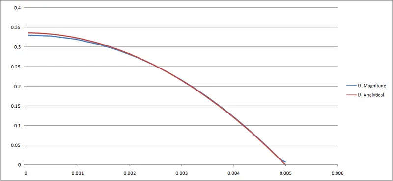
Image 3.4 Analytical and Simulation Velocity Profile.
In the above graph, the velocity profile is nearly the same and there is a slight difference near the wall and the axis. This is due to the coarse mesh, the finer the mesh accurate the results. Since the simulation is done on the wedge there is only half of the velocity profile i.e from the axis to the wall. The fluid velocity in a pipe changes from zero at the wall because of the no-slip condition to a maximum at the pipe center. In fluid flow, it is convenient to work with an average velocity Vavg, which remains constant in incompressible flow when the cross-sectional area of the pipe is constant(refer to image 1.1). The maximum velocity of the flow is 0.3299m/s which is almost double the average velocity as described in the Fluid Dynamics Textbook.
Plotting the Pressure Difference along the length when the flow is fully developed:
The same command is used to plot the Pressure Difference but it is plotted along the x-direction after the entrance length(i.e from 1.1m to 1.2m). It is plotted after the entrance length as the flow is fully developed after the entrance length. The pressure obtained from the simulation is Kinematic Pressure and to obtain the static pressure it is multiplied with density of the fluid(water).
Static Pressure `p_s` = `p_krho`
`p_s = 0.00438596xx995`
`p_s = 4.364 Pa`
The pressure difference for a fully developed flow i.e at distance from 1.1m to 1.2m was found to be 4.364 Pa from the simulation and 4.2897 from the analytical solution i.e from Hagen- Poiseuille's Equation.
`trianglep = (8muLV_(avg))/R^2`
`trianglep =( 8xx0.000797xx0.1xx0.1682)/0.005^2`
`trianglep = 4.2897Pa`
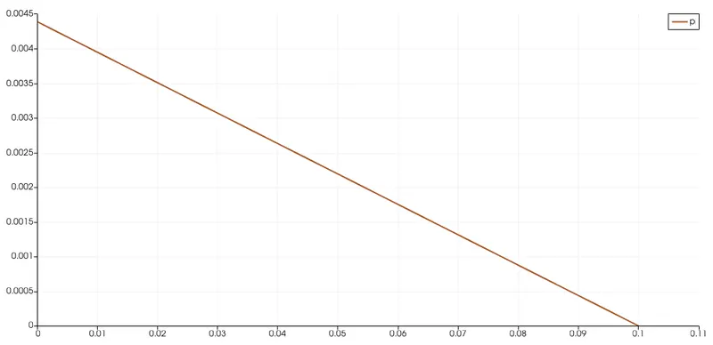
Image 3.5 Pressure Difference
Plotting the Shear Force along the radial distance:
Shear Force = `mu(delU)/(delx`
Using the calculator tool in the ParaView first magnitude of velocity is calculated and using the GradientofUnstructureData tool the gradient of velocity is calculated and again the calculator tool is used to calculate the Shear force.
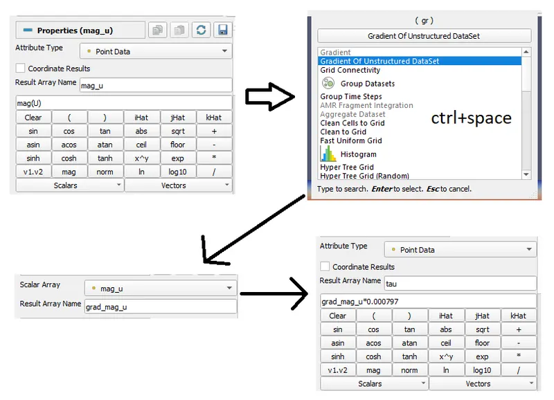
Image 3.6 Shear Force Plotting Procedure
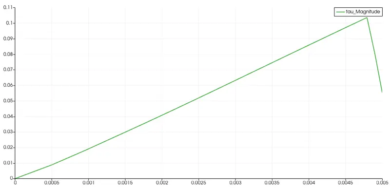
Image 3. Shear Force Profile.
From the graph, it is seen that the shear force increase exponentially from the axis towards the wall and there is drop near the axis. This drop in the shear force is due to the no-slip condition i.e the layer of fluid in contact with the wall has zero velocity(stationary) and the layer of fluid next to that layer is in motion. The Maximum Shear force was found to be 0.11836 N.
CONCLUSION:
1. The axis-symmetric steady, incompressible, laminar(Reynolds Number = 2100) flow by applying the wedge boundary condition simulated using the icoFoam solver in OpenFOAM and the results are viewed in ParaView.
2. The results are also validated with Hagen- Poiseuille's equations for the fully developed flow.
| Simulation Results | Analytical Results | |
| Maximum Velocity | 0.336 m/s | 0.329 m/s |
| Pressure Difference for fully developed flow. | 4.364 Pa | 4.289 Pa |
The Maximum Shear stress was found to be 0.11836N from the simulation
3. A code in MATLAB to automate the generation of blockMeshDict file is developed and it takes pipe length, diameter, wedge angle as input and gives a fully functional blockMeshDict file.