Simulation of Laminar Flow through a pipe in OpenFoam
I. Aim: To simulate incompressible laminar pipe flow in OpenFoam.
II Problem Statement:
Simulate an axisymmetric flow by applying the wedge boundary condition. The flow is laminar and flows through a constant cross-section pipe at an inlet Reynold's number of 2100. Perform a transient or steady-state simulation and validate numerical results with the Hagen- Poiseuille's equations for the fully developed flow.
Write a code in Matlab to automate the generation of blockMeshDict file. The code should take inputs like pipe length, diameter, wedge angle, etc, and output a fully functional blockMeshDict file.
Expected Results
- Validate Hydro-dynamic length with the numerical result
- Validate the fully developed flow velocity profile with its analytical profile
- Validate maximum velocity and pressure drop for fully developed flow
- Post-process Shear stress and validate wall shear stress for fully developed flow.
Theory:
The flow through a circular pipe can be divided into two regions from the inlet to the outlet namely :
1. Hydrodynamic entrance region
2. Fully developed flow region
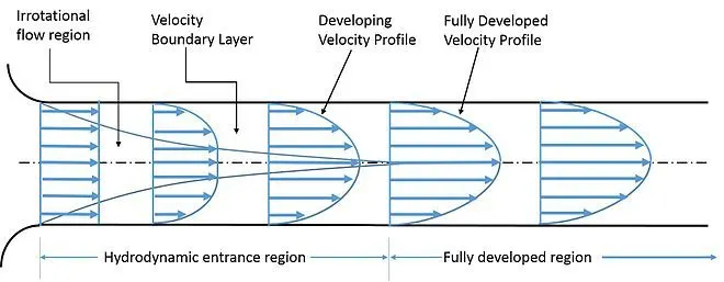
In the hydrodynamic entrance region, the flow develops with an increase in velocity boundary layer thickness along the pipe length due to viscous effects. The hydrodynamic entrance length is the distance from the inlet of the pipe along the pipe length where the two velocity boundary layers from the bottom and top side of the pipe meet at the centerline of the pipe as shown in the above figure. Theoretically, the hydrodynamic entrance length for a laminar flow through a pipe is given by the relation:
`L_(h,lam) = 0.06*Re*D` ........................(1)
where, Re = flow Reynolds number
D = pipe diameter
The flow after the hydrodynamic entrance region is called a fully developed region due to the presence of fully developed velocity boundary layers. The velocity profile is parabolic in nature in the fully developed region. The fully developed viscous laminar flow (Re<2300) through a pipe is described as Hagen-Poiseuille flow.
The analytical equations describing the Hagen-Poiseuille flow through a pipe are given below:
1. velcoity variation at a cross section:
`V = 1/(4mu)*(dp)/dx*(R^2-r^2)`
2. Average velocity, `V_(avg)=1/(8mu)*(dp)/dx*R^2`
3. Maximum velocity , `V_max = 2*V_(avg)`
4. Pressure drop along the pipe, `Deltap = (32muV_(avg)L)/D^2`
5. Wall shear stress , `tau = -(dp)/dx*(R/2)`
where, R= radius of the pipe = D/2
`mu` = Dynamic viscosity of the fluid
L = length of the fully developed pipe section under consideration.
III. Objectives:
1. Simulate a 2D axisymmetric laminar pipe flow(Re = 2100) by applying the wedge boundary condition.
2. Write a code in Matlab to automate the generation of blockMeshDict file.
3. Validate numerical results with analytical results.
Inputs Considered:
1. Lenght of the pipe, L = 1000 mm.
2. Dia of the pipe , D = 5 mm
3. Inlet Reynolds number , Re = 2100
4. Fluid considered is water , density `rho = 1000 (kg)/m^3`;
kinematic viscosity, `mu = 7.978e^-4 Pa.s`
kinematic viscosity, `nu = 7.978e^-7 m^2/s`
5. Inlet velocity , `V = (Re.nu)/D`= 0.336 m/s
6. Hydrodynamic entrance length , `L_(h,lam)` = 0.63 m;
7. Fully developed region length, `L_(FDR) = L- L_(h,lam) = 0.37 m`
Analytical values:
The analytical results computed using Hagen-Poiseuille flow equations for the above-mentioned input parameters.
1. Average velocity, `V_(avg) = 0.336 m/s`
2. Maximum velocity , `V_max = 2.V_(avg)` = 0.672 m/s.
3. pressure drop in the fully developed region , `Deltap = 126.95 Pa`
4. `((dp)/dx) = (Deltap)/L_(FDR) = 343.1 Pa`
4. Wall shear stress , `tau = 0.428 N/m^2`
IV. Numerical Solution:
The numerical analysis is carried out using 'icofoam' solver in OpenFoam, which is an incompressible laminar flow solver. A 2D axi-symmetric analysis is carried out, with the wedge type boundaries along the tangential direction as shown below:
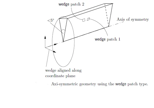
A wedge angle of 3 degrees is considered for the analysis.
Boundary types:
1. Inlet: type patch
2. Outlet: type patch
3. Wedges: type Wedges
4. Axis: type empty
6. Wall : type noSlip
In order to automate the mesh generation, Matlab code is executed to generate the blockMeshDict file. The code for the same is shown below:
Matlab code for generating blockMeshDict file.
%Script code for generating blockMeshDict file for 2d axisymmetric flow through a pipe in openFOAM

close all
clear all
clc

%input parameters of domain
a = input('Enter the length of the pipe in mm =');
b = input('Enter the diameter of the pipe in mm =');
c = input('Enter the wedge angle in degrees =');
d = input('Enter the number of mesh cells along axial direction = ');
e = input('Enter the number of mesh cells along radial direction = ');
f = input('Enter the number of mesh cells points along tangential direction = ');
g = input('Enter the mesh expansion ratio along axial direction = ');
h = input('Enter the mesh expansion ratio along radial direction = ');
i = input('Enter the mesh expansion ratio along tangential direction = ');


%Meshfile
A = fopen('blockMeshDict.txt','w')
%header content
fprintf(A,'/*---------------------------------------*- C++ -*-----------------------------------------*');
fprintf(A,'n  =========                     |');
fprintf(A,'n  \      /  F ield             | OpenFOAM: The Open Source CFD Toolbox');
fprintf(A,'n   \    /   O peration         | Website:  https://openfoam.org');
fprintf(A,'n    \  /    A nd               | version:  8');
fprintf(A,'n     \/     M anipulation      | ');
fprintf(A,'n*---------------------------------------*- C++ -*-----------------------------------------*/');

fprintf(A,'nFoamFile');
fprintf(A,'n{');
fprintf(A,'n    version    2.0;');
fprintf(A,'n    format     ascii;');
fprintf(A,'n    class      dictionary;');
fprintf(A,'n    object     blockMeshDict;');
fprintf(A,'n}');
fprintf(A,'n//* * * * * * * * * * * * * * * * * * * * //');
fprintf(A,'n');
fprintf(A,'nconvertToMeters 0.001;');
fprintf(A,'n');

%vertices
fprintf(A,'nvertices');
fprintf(A,'n(');
fprintf(A,'n  (0 0 0)      //0-vertex at inlet_center_point');
fprintf(A,'n  (0 %d %d)      //1-second vertex at inlet',(b/2*cosd(c/2)),(b/2*sind(c/2)));
fprintf(A,'n  (0 %d %d)      //2-third vertex at inlet',(b/2*cosd(c/2)),(-b/2*sind(c/2)));
fprintf(A,'n  (%d 0 0)      //3-vertex at outlet_center_point',a);
fprintf(A,'n  (%d %d %d)      //4-second vertex at outlet',a,(b/2*cosd(c/2)),(b/2*sind(c/2)));
fprintf(A,'n  (%d %d %d)      //5-third vertex at inlet',a,(b/2*cosd(c/2)),(-b/2*sind(c/2)));
fprintf(A,'n);');

%edges
fprintf(A,'nedges');
fprintf(A,'n(');
fprintf(A,'n  arc 1 2 3 (0 1 0)   // inlet arc from vertex 1 to vertex 2,3 degrees, y-normal');
fprintf(A,'n  arc 4 5 3 (0 1 0)   // outlet arc from vertex 4 to vertex 5, 3 degrees, y-normal');
fprintf(A,'n);');
%blocks
fprintf(A,'nblocks');
fprintf(A,'n(');
fprintf(A,'n  hex (0 2 1 0 3 5 4 3) (%d %d %d) simpleGrading (%d %d %d)  // wedge',e,f,d,h,i,g);
fprintf(A,'n);');
%boundaries
fprintf(A,'nboundary');
fprintf(A,'n(');
%inlet
fprintf(A,'n      inlet  // inlet boundary');
fprintf(A,'n{');
fprintf(A,'n      type patch;');
fprintf(A,'n      faces');
fprintf(A,'n      (');
fprintf(A,'n      (0 2 1 0)');
fprintf(A,'n      );');
fprintf(A,'n}');
%outlet
fprintf(A,'n      outlet  // outlet boundary');
fprintf(A,'n{');
fprintf(A,'n      type patch;');
fprintf(A,'n      faces');
fprintf(A,'n      (');
fprintf(A,'n      (3 5 4 3)');
fprintf(A,'n      );');
fprintf(A,'n}');
%wall
fprintf(A,'n      noslipwall  // wall boundary');
fprintf(A,'n{');
fprintf(A,'n      type noSlip;');
fprintf(A,'n      faces');
fprintf(A,'n      (');
fprintf(A,'n      (1 2 5 4)');
fprintf(A,'n      );');
fprintf(A,'n}');

%wedges
fprintf(A,'n      wedge1  // wedge');
fprintf(A,'n{');
fprintf(A,'n      type wedge;');
fprintf(A,'n      faces');
fprintf(A,'n      (');
fprintf(A,'n      (0 1 4 3)');
fprintf(A,'n      );');
fprintf(A,'n}');


fprintf(A,'n      wedge2  // wedge');
fprintf(A,'n{');
fprintf(A,'n      type wedge;');
fprintf(A,'n      faces');
fprintf(A,'n      (');
fprintf(A,'n      (0 2 5 3)');
fprintf(A,'n      );');
fprintf(A,'n}');

%axis
fprintf(A,'n      axis  // centerline');
fprintf(A,'n{');
fprintf(A,'n      type empty;');
fprintf(A,'n      faces');
fprintf(A,'n      (');
fprintf(A,'n      (0 3 3 0)');
fprintf(A,'n      );');
fprintf(A,'n}');
fprintf(A,'n);');

%matchinhg patches
fprintf(A,'nmergePatchPairs   // merging matching faces');
fprintf(A,'n(');
fprintf(A,'n);');

fprintf(A,'n');
fprintf(A,'n//************************************************//');


fclose(A);
In-order to check the effect of mesh size on the results three different meshes were used:
| Number of cells (axial,radial,tangential) |
Grading Factor (axial,radial,tangential) |
|
| Case1 | (500,20,1) | (1,0.3,1) |
| Case2 | (500,40,1) | (1,0.3,1) |
| Case3 | (500,80,1) | (1,0.1,1) |
The blockMeshDict file for case3 generated by Matlab coding is shown below:
/*---------------------------------------*- C++ -*-----------------------------------------*
  =========                     |
        /  F ield             | OpenFOAM: The Open Source CFD Toolbox
       /   O peration         | Website:  https://openfoam.org
      /    A nd               | version:  8
     /     M anipulation      |
*---------------------------------------*- C++ -*-----------------------------------------*/
FoamFile
{
    version    2.0;
    format     ascii;
    class      dictionary;
    object     blockMeshDict;
}
//* * * * * * * * * * * * * * * * * * * * //

convertToMeters 0.001;

vertices
(
  (0 0 0)      //0-vertex at inlet_center_point
  (0 2.499143e+00 6.544237e-02)      //1-second vertex at inlet
  (0 2.499143e+00 -6.544237e-02)      //2-third vertex at inlet
  (1000 0 0)      //3-vertex at outlet_center_point
  (1000 2.499143e+00 6.544237e-02)      //4-second vertex at outlet
  (1000 2.499143e+00 -6.544237e-02)      //5-third vertex at inlet
);
edges
(
  arc 1 2 3 (0 1 0)   // inlet arc from vertex 1 to vertex 2,3 degrees, y-normal
  arc 4 5 3 (0 1 0)   // outlet arc from vertex 4 to vertex 5, 3 degrees, y-normal
);
blocks
(
  hex (0 2 1 0 3 5 4 3) (80 1 500) simpleGrading (1.000000e-01 1 1)  // wedge
);
boundary
(
      inlet  // inlet boundary
{
      type patch;
      faces
      (
      (0 2 1 0)
      );
}
      outlet  // outlet boundary
{
      type patch;
      faces
      (
      (3 5 4 3)
      );
}
      noslipwall  // wall boundary
{
      type noSlip;
      faces
      (
      (1 2 5 4)
      );
}
      wedge1  // wedge
{
      type wedge;
      faces
      (
      (0 1 4 3)
      );
}
      wedge2  // wedge
{
      type wedge;
      faces
      (
      (0 2 5 3)
      );
}
      axis  // centerline
{
      type empty;
      faces
      (
      (0 3 3 0)
      );
}
);
mergePatchPairs   // merging matching faces
(
);

//************************************************//
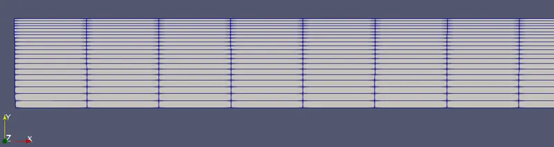
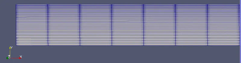
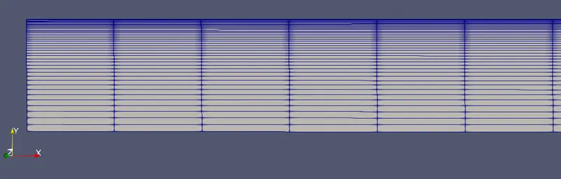
The meshes generated by executing the blockMesh command and viewing in paraview using paraFoam command are shown below:
Case1:
| Axial direction of the pipe | Cross section view |
 |
 |
Case2:
| Axial direction of the pipe | Cross section view |
 |
 |
Case3:
| Axial direction of the pipe | Cross section view |
 |
 |
The initial and boundary conditions for the domain used for the numerical analysis are shown in the below initial condition files for pressure and velocity.
1. Inlet :
Velocity - Uniform , value = 0.336 m/s
pressure - zeroGradient.
2. Outlet
Velocity - zeroGradient
Pressure - Uniform , Value = 0.12695 m (The pressure at the outlet is defined in terms of kinematic pressure(`(Deltap)/rho`,m) having the value equal to the pressure drop in the fully developed section)
3. Wedges - Type wedge;
4. axis - type empty
5. noslip wall
Velocity - type noSlip;
Pressure - type - uniform.
Velocity:
/*--------------------------------*- C++ -*----------------------------------*
  =========                 |
        /  F ield         | OpenFOAM: The Open Source CFD Toolbox
       /   O peration     | Website:  https://openfoam.org
      /    A nd           | Version:  8
     /     M anipulation  |
*---------------------------------------------------------------------------*/
FoamFile
{
    version     2.0;
    format      ascii;
    class       volVectorField;
    object      U;
}
// * * * * * * * * * * * * * * * * * * * * * * * * * * * * * * * * * * * * * //

dimensions      [0 1 -1 0 0 0 0];

internalField   uniform (0 0 0);

boundaryField
{
    inlet
    {
        type            fixedValue;
        value           uniform (0.336 0 0);
    }

    noslipwall
    {
        type            noSlip;
    }
    wedge1
    {
    	type 		 wedge;
    }
    wedge2
    {
    	type 		 wedge;
    }
    axis
    {
    	type 		 empty;
    }
    outlet
    {
        type            zeroGradient;
    }
}

// ************************************************************************* //
Pressure:
/*--------------------------------*- C++ -*----------------------------------*
  =========                 |
        /  F ield         | OpenFOAM: The Open Source CFD Toolbox
       /   O peration     | Website:  https://openfoam.org
      /    A nd           | Version:  8
     /     M anipulation  |
*---------------------------------------------------------------------------*/
FoamFile
{
    version     2.0;
    format      ascii;
    class       volScalarField;
    object      p;
}
// * * * * * * * * * * * * * * * * * * * * * * * * * * * * * * * * * * * * * //

dimensions      [0 2 -2 0 0 0 0];

internalField   uniform 0;

boundaryField
{
    inlet
    {
        type            zeroGradient;
    }

    noslipwall
    {
        type            zeroGradient;
    }
    wedge1
    {
    	type 		 wedge;
    }
    wedge2
    {
    	type 		 wedge;
    }
    axis
    {
    	type 		 empty;
    }
    outlet
    {
        type            fixedValue;
        value		 uniform 0.12695;
    }
}

// ************************************************************************* //
Transport properties:
/*--------------------------------*- C++ -*----------------------------------*
  =========                 |
        /  F ield         | OpenFOAM: The Open Source CFD Toolbox
       /   O peration     | Website:  https://openfoam.org
      /    A nd           | Version:  8
     /     M anipulation  |
*---------------------------------------------------------------------------*/
FoamFile
{
    version     2.0;
    format      ascii;
    class       dictionary;
    location    "constant";
    object      transportProperties;
}
// * * * * * * * * * * * * * * * * * * * * * * * * * * * * * * * * * * * * * //

nu              [0 2 -1 0 0 0 0] 7.978e-7;


// ************************************************************************* //
A time duration 3 seconds and a Courant number of 0.1 is considered for the transient analysis. The timestep for the three cases of mesh sizes given below:
`Deltat = (C*nu)/V_max`
| timestep(`Deltat`) | |
| Case1 | 2.976e-4 |
| Case2 | 1.488e-4 |
| Case3 | 1.488e-4 |
The time duration and the timestep size are defined in the controlDict file.
controlDictfile:
/*--------------------------------*- C++ -*----------------------------------*
  =========                 |
        /  F ield         | OpenFOAM: The Open Source CFD Toolbox
       /   O peration     | Website:  https://openfoam.org
      /    A nd           | Version:  8
     /     M anipulation  |
*---------------------------------------------------------------------------*/
FoamFile
{
    version     2.0;
    format      ascii;
    class       dictionary;
    location    "system";
    object      controlDict;
}
// * * * * * * * * * * * * * * * * * * * * * * * * * * * * * * * * * * * * * //

application     icoFoam;

startFrom       startTime;

startTime       0;

stopAt          endTime;

endTime         3;

deltaT          0.0001488;

writeControl    timeStep;

writeInterval   20;

purgeWrite      0;

writeFormat     ascii;

writePrecision  6;

writeCompression off;

timeFormat      general;

timePrecision   6;

runTimeModifiable true;


// ************************************************************************* //
Numerical results:
The steady-state results of the analysis from the 'icofoam' solution post-processed in paraview are discussed below:
1: Velocity Profiles:
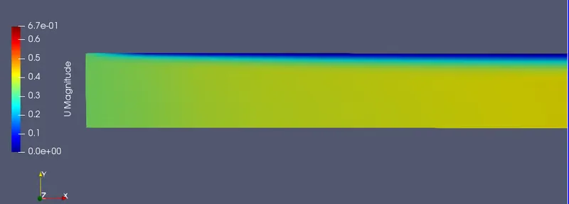
Figure1: Velocity contour at the inlet side of the pipe.
The above contour plot represents the velocity magnitude variation at the inlet section of the 2D axisymmetric pipe. It can be observed at the entry of the pipe(inlet), the velocity is equal across the cross-section (v = 0.336 m/s) which is the inlet boundary condition specified. As the flow moves along the pipe the hydrodynamic boundary layer develops and grows in size, which is seen in the plot as the blue region. The velocity near to the wall is approaching zero magnitude due to viscosity and no-slip conditions.
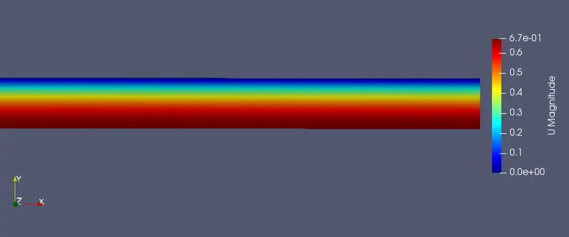
Figure2: Velocity contour at the outlet side of the pipe (Fully developed flow section).
The above contour plot represents the velocity magnitude variation near the outlet section of the 2D axisymmetric pipe, which is in the fully developed section of the flow. It can be observed the velocity at the centerline of the pipe (axis) is maximum (v = 0.672 m/s) which is twice the average velocity of the flow(0.336 m/s). The boundary layer has fully developed in this section and there is no further growth in its size as evident from the constant blue region along the pipe.
Velocity profile variation along the pipe length:
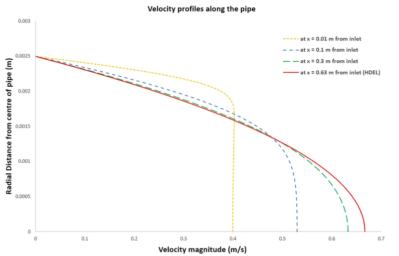
The above plot shows the velocity profile at various distances from the inlet. The velocity profile is different at each cross-section, with the profile at x =0.63 m having a parabolic profile and maximum velocity of 0.665 m/s. The value is almost equal to the analytical value (V_max = 0.672 m/s). This indicates the flow has fully developed and the cross-section is the hydro_dynamic entrance (x =0.63m). This is equal to the analytical hydrodynamic entrance length (`L_(h,lam) = 0.63 m`.
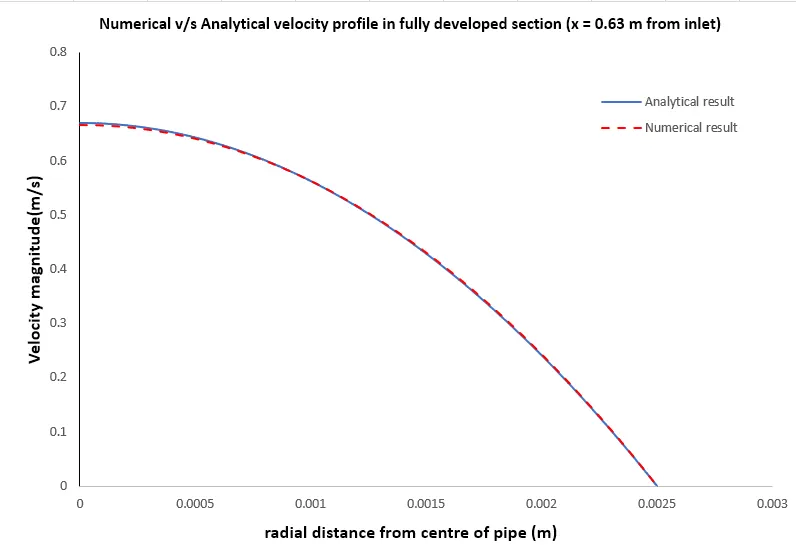
The above plot represents the validation of the velocity profile in the fully developed flow region (x =0.63 m) with that of the analytical velocity profile. The velocity is maximum at the centreline(axis) and approaches zero near the wall. It can be seen that the numerical solution is in good agreement with the analytical result.
2. Pressure:
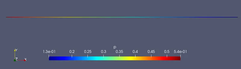
Figure 3: Pressure variation along the pipe.
Pressure drop in the fully developed section:
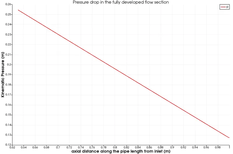
The pressure drop in the fully developed region of the pipe is shown in the above plot. The pressure(kinematic pressure) at the fully developed flow entrance is calculated as part of the solution and it drops to 0.1269 m at the outlet which is the boundary condition. It can be seen that the pressure drops from 0.254 m at x =0.63 m to 0.1269 m at the outlet. The difference is equal to 0.127, which is almost equal to the analytical pressure drop calculated from the Hagen_Poiseullie equation. Hence the numerical result is in good agreement with the analytical result.
3. Shear stress:
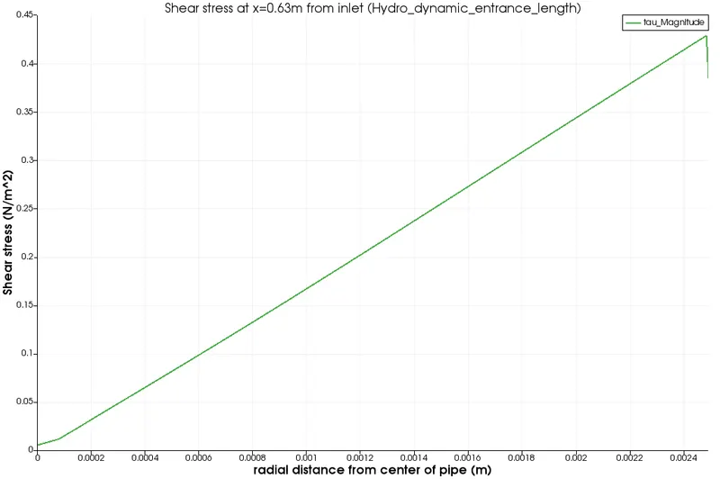
The above plot represents the variation of shear stress from the centerline (axis) to the wall of the pipe in the fully developed region. It can be seen that the shear stress is maximum at the wall and at least the axis of the pipe. The shear stress varies linearly. The maximum shear stress is at the wall and is equal to 0.428 N/m^2. This value is equal to the analytical value of wall shear stress(0.428 N/m^2).
Note: The above-mentioned contours, plots are for the Case3 mesh properties.
Validation of Numerical results:
| Analytical results (Hagen-Poiseiulle equations) | Numerical results | error (%) | |||||
| Parameter | case 1 | case2 | case3 | case1 | case2 | case3 | |
| Max Velocity (m/s) | 0.672 | 0.665 | 0.6661 | 0.66645 | 1.04 | 0.825 | 0.825 |
| Pressure drop (Pa) | 126.95 | 127.4 | 127.32 | 127.21 | 0.35 | 0.204 | 0.204 |
| Wall Shear stress | 0.427 | 0.365 | 0.414 | 0.428 | 14.5 | 3.04 | 0.234 |
The above table shows the effect of mesh size on the numerical results values. The numerical results are in good agreement with the analytical results. The pressure drop and maximum velocity in the fully developed region (x =0.63 m) agreed well in the cas1 and case2 mesh parameters with the analytical results, but the wall shear stress showed a lot of deviation from the analytical results. The mesh is made very fine in case3 near the wall which resulted in the numerical wall shear stress matching the analytical result.
Conclusion:
The objective of this project is to simulate the 2D axisymmetric laminar flow in a pipe in OpenFOAM. It is observed that the velocity boundary layer develops up to the entrance length, thereafter it becomes constant. The maximum velocity occurs at the centerline of the pipe and the maximum shear stress is at the wall. The numerical results are in good agreement with the analytical results from Hagen_Poiseullie flow equations. The velocity has a parabolic profile in the fully developed region. The pressure drops linearly in the fully developed region. The near-wall mesh refinement improves the wall results like shear stress.