Week 11 - Simulation of Flow through a pipe in OpenFoam
Objective:
a) To simulate an axi-symmetrix flow by applying wedge boundary condition for a laminar flow through a pipe of constant diamter .
b) Write a code in matlab to auto-generate the blockMeshDict file for this simulation .
c)
- Validate Hydro-dynamic length with the numerical result
- Validate the fully developed flow velocity profile with its analytical profile
- Validate maximum velocity and pressured drop for fully developed flow
- Post-process Shear stress and validate wall shear stress for fully developed flow
Theory :
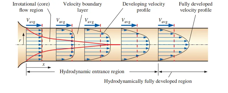
Consider a fluid entering a circular pipe at uniform vellocity . Because of the no-slip condition , fluid particles in contact with the wall of the pipe, come to a complete stop . This layer causes the fluid particles in the adjacent layers to slow down as well due to friction . To make up for this velocity reduction, the velocity of the fluid at the midsection has to increase in order to keep the mass flow rate constant in the pipe . As a result, veocity gradient forms along the pipe .
The region of the flow in which , the effects of the viscous shearing forces caused by fluid viscosity are felt , is called velocity boundary layer or just boundary layer. The hypothetical boundary layer divides the flow into 2 region : the boundary layer region (viscous effects and velocity changes are significant )and the irrotational flow region (frictional effects are insignificant and velocity remains constant in radial direction).
The thickness of the boundary layer increase in the flow direction till the boundary layer reaches the pipe centre and thus fills the entire pipe and the velocity becomes fully develped a little farther downstream . The region from the pipe entrance to the region till which the velocity profile is fully formed is called hydrodynamic entrance region and the length of this region is called hydrodynamic entry length `L_h`. Flow iin the entry region is called hydrodynamically developing flow since this is the region in which the velocity profile is developing . The region beyond which the velocity profile is fully developed is called hydrodynamically fully developed region . The flow is said to be fully developed when the normalized temperature profile remains unchanged. The velocity profile in laminar fully developed flow in parabolic and much flatter in turbulent flow because of the formation of eddys and vigorous mixing of radial direction . The time averaged velocity profile remains unchanged when the flow is fully developed .
`(delu)/(delx)(r,x) = 0 -> u=u(r)`
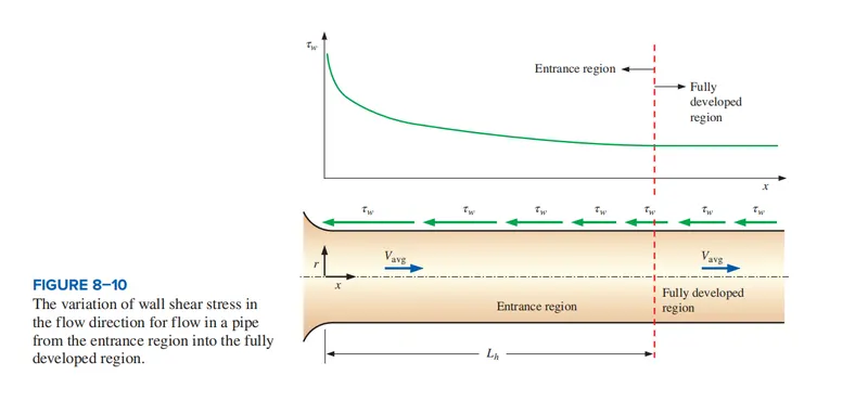
The shear stress at pipe wall `tau_w` is related to the slope of the velocity profile at the surface . Consider the fluid flow in hydrodynamic entrance region of the pipe . The wall shear stress is highest at the inlet region of the pipe where thickness of boundary layer is minimum and decreases gradually to fully developed region. Therefore the pressure drop is always higher in the entrance region of the pipe and the effect of the entrance region always increases the average friction factor for the entire pipe . This increase may be significant for short pipes, but is negligible for long pipes.
Given below is the equation for hydrodynamic length for flow of Re<2300 .
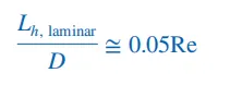
`L_h= .05*Re*D` = .05x2100x.005 = 0.525m
where D is the diameter of the pipe. (assumed value)
Total length of the pipe we consider = L>Lh = 0.1xRexD = 1.05m
Given below is graph for variation of wall shear stress along the hydrodynamic length of a pipe .
Given below are equations for pressure drop and average velocity for an incompressible laminar flow through a pipe .
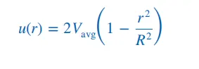
where r/R is the ratio of radius from centre to circumference of the pipe .
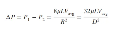
Where
`mu` is the dynamic viscosity
L is the length of the pipe
Vavg = average velocity
D = Diameter of the pipe .
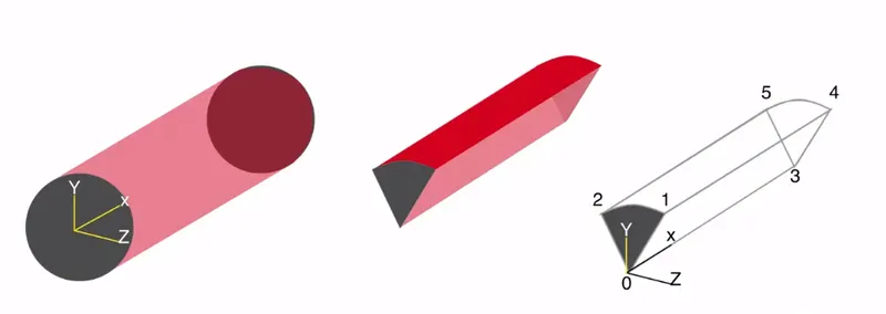
In this case , in order to simplify the calculations , we reduce the pipe into a wedge with wedge angle 3 degrees . This would enable us to reduce the computation time without compromising on the accuracy of the results .
Programe Codes :
1) Matlab code to automate creation of block mesh .
clear all
close all
clc

D=.005 ;
r=D/2 ;
L= 210*D ;
Re=2100 ;
theta=3 ;
a=sin(theta/2);
b=cos(theta/2);
y=r*a;
z=r*b;

f1=fopen('blockMeshDict.txt','w');
fprintf(f1," /*--------------------------------*- C++ -*----------------------------------* \n " );
fprintf(f1,"  =========                 | /n " );
fprintf(f1,"  \\      /  F ield         | OpenFOAM: The Open Source CFD Toolbox \n");
fprintf(f1,"   \\    /   O peration     | Website:  https://openfoam.org \n");
fprintf(f1,"    \\  /    A nd           | Version:  8 \n");
fprintf(f1,"     \\/     M anipulation  |  \n");
fprintf(f1,"*---------------------------------------------------------------------------* \n");
fprintf(f1,"FoamFile \n");
fprintf(f1," { \n");
fprintf(f1,"    version     2.0; \n");
fprintf(f1,"    format      ascii; \n");
fprintf(f1,"    class       dictionary; \n ");
fprintf(f1,"    object      blockMeshDict; \n" );
fprintf(f1,"   } \n");
fprintf(f1,"// * * * * * * * * * * * * * * * * * * * * * * * * * * * * * * * * * * * * * // \n");

fprintf(f1,"convertToMeters 1; \n");

fprintf(f1,"vertices \n");
fprintf(f1,"( \n");
fprintf(f1,"   (0 0 0) \n");                         % Vertex 0
fprintf(f1,"   (0 %d %d ) \n",y,z);                  % Vertex 1
fprintf(f1,"   (0 %d %d) \n",y,-z);                  % Vertex 2
fprintf(f1,"   (%d 0 0) \n",L);                      % Vertex 3
fprintf(f1,"   (%d %d %d) \n",L,y,z);                % Vertex 4
fprintf(f1,"   (%d %d %d))\n",L,y,-z);               % Vertex 5

fprintf(f1,"  ); \n");

fprintf(f1,"blocks \n");
fprintf(f1," ( \n ");
fprintf(f1,"   hex (0 3 5 2 0 3 4 1) (200 50 1) simpleGrading (1 .1 1) \n");
fprintf(f1," ); \n");

fprintf(f1," edges \n ");
fprintf(f1," ( \n ");
fprintf(f1," ); \n ");

fprintf(f1," boundary \n");
fprintf(f1," ( \n " );
fprintf(f1,"   inlet \n ");
fprintf(f1,"   {   \n ");
fprintf(f1,"       type wall; \n");
fprintf(f1,"       faces \n");
fprintf(f1,"       (  \n");
fprintf(f1,"           (0 1 2 0) \n");
fprintf(f1,"       );  \n");
fprintf(f1,"   }  \n");
fprintf(f1,"  Outlet \n ");
fprintf(f1,"   {   \n ");
fprintf(f1,"       type wall; \n");
fprintf(f1,"       faces \n");
fprintf(f1,"       (  \n");
fprintf(f1,"           (3 5 4 3  ) \n");
fprintf(f1,"       );  \n");
fprintf(f1,"   }  \n");

fprintf(f1,"  topWall \n");
fprintf(f1,"    {  \n");
fprintf(f1,"        type wall;  \n");
fprintf(f1,"        faces \n");
fprintf(f1,"        (  \n");
fprintf(f1,"            (1 4 5 2) \n");
fprintf(f1,"        ); \n");
fprintf(f1,"    }  \n");
fprintf  (f1,"  axis \n");
fprintf(f1,"    {  \n");
fprintf(f1,"        type empty;  \n");
fprintf(f1,"        faces \n");
fprintf(f1,"        (  \n");
fprintf(f1,"            (0 3 3 0 ) \n");
fprintf(f1,"        ); \n");
fprintf(f1,"    }  \n");
fprintf(f1,"    front \n");
fprintf(f1,"    { \n");
fprintf(f1 ,"      type wedge;\n");
fprintf(f1,"       faces   \n");
fprintf(f1,"       ( \n");
fprintf(f1,"           (0 3 4 1) \n");
fprintf(f1,"       ); \n");
fprintf(f1,"   } \n");
fprintf(f1,"    back \n");
fprintf(f1,"    { \n");
fprintf(f1 ,"      type wedge;\n");
fprintf(f1,"       faces   \n");
fprintf(f1,"       ( \n");
fprintf(f1,"           (0 2 5 3) \n");
fprintf(f1,"       ); \n");
fprintf(f1,"   } \n");
fprintf(f1,"); \n");

fprintf(f1,"mergePatchPairs \n");
fprintf(f1,"( \n");
fprintf(f1,"); \n");

fprintf(f1,"// ************************************************************************* // ");
Code for pressure initial and boundary conditions .
/*--------------------------------*- C++ -*----------------------------------*\
  =========                 |
  \\      /  F ield         | OpenFOAM: The Open Source CFD Toolbox
   \\    /   O peration     | Website:  https://openfoam.org
    \\  /    A nd           | Version:  8
     \\/     M anipulation  |
\*---------------------------------------------------------------------------*/
FoamFile
{
    version     2.0;
    format      ascii;
    class       volScalarField;
    object      p;
}
// * * * * * * * * * * * * * * * * * * * * * * * * * * * * * * * * * * * * * //

dimensions      [0 2 -2 0 0 0 0];

internalField   uniform 0;

boundaryField
{
     inlet
    {
        type            zeroGradient;
    }

    Outlet
    {
        type            fixedValue;
        value           uniform 0 ;
    }

    topWall
    {
    type                zeroGradient;
    }

    axis
    {
    type                  empty;
    }

    front
    {
        type            wedge;
    }

    back
    {
        type            wedge;
    }


}

// ************************************************************************* //
Code for velocity Initial and boundary conditions
/*--------------------------------*- C++ -*----------------------------------*\
  =========                 |
  \\      /  F ield         | OpenFOAM: The Open Source CFD Toolbox
   \\    /   O peration     | Website:  https://openfoam.org
    \\  /    A nd           | Version:  8
     \\/     M anipulation  |
\*---------------------------------------------------------------------------*/
FoamFile
{
    version     2.0;
    format      ascii;
    class       volVectorField;
    object      U;
}
// * * * * * * * * * * * * * * * * * * * * * * * * * * * * * * * * * * * * * //

dimensions      [0 1 -1 0 0 0 0];

internalField   uniform (0 0 0);

boundaryField
{
     inlet
    {
        type            fixedValue;
        value           uniform (0.42 0 0);
    }

     Outlet
    {
        type               zeroGradient;
    }
     topWall
     {
     type              noSlip;
     value             uniform (0 0 0);
     }

     axis
     {
     type              empty;
     }

    front
    {
        type            wedge;
    }

    back
    {
    type                wedge;
    }
}

// ************************************************************************* //
Code for controlDict
/*--------------------------------*- C++ -*----------------------------------*\
  =========                 |
  \\      /  F ield         | OpenFOAM: The Open Source CFD Toolbox
   \\    /   O peration     | Website:  https://openfoam.org
    \\  /    A nd           | Version:  8
     \\/     M anipulation  |
\*---------------------------------------------------------------------------*/
FoamFile
{
    version     2.0;
    format      ascii;
    class       dictionary;
    location    "system";
    object      controlDict;
}
// * * * * * * * * * * * * * * * * * * * * * * * * * * * * * * * * * * * * * //

application     icoFoam;

startFrom       startTime;

startTime       0;

stopAt          endTime;

endTime         3;

deltaT          0.0001;

writeControl    timeStep;

writeInterval   20;

purgeWrite      0;

writeFormat     ascii;

writePrecision  6;

writeCompression off;

timeFormat      general;

timePrecision   6;

runTimeModifiable true;


// ************************************************************************* //
Output :
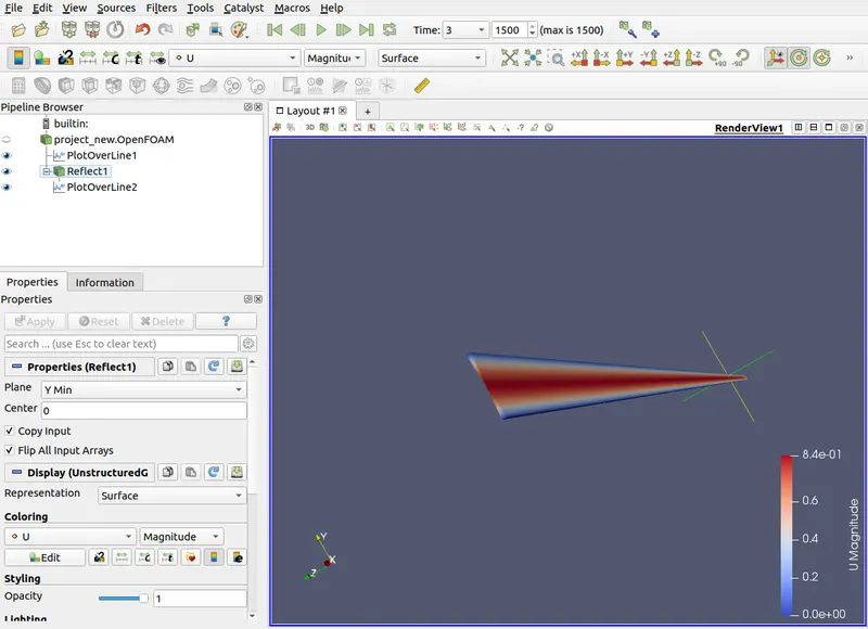
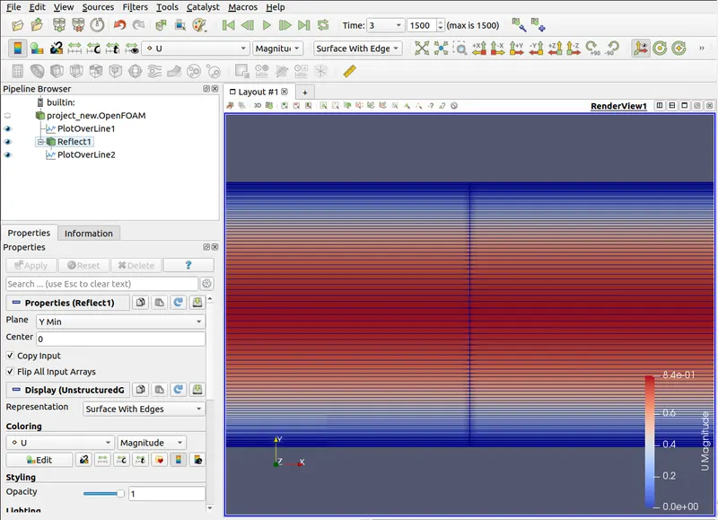
1) The axi-symmetric flow was simulated and paraFoam view of the wedge was obtained .
Shown below is a reflected render of the wedge in order to obtain a full velocity profile.
1)Velocity profile obtained
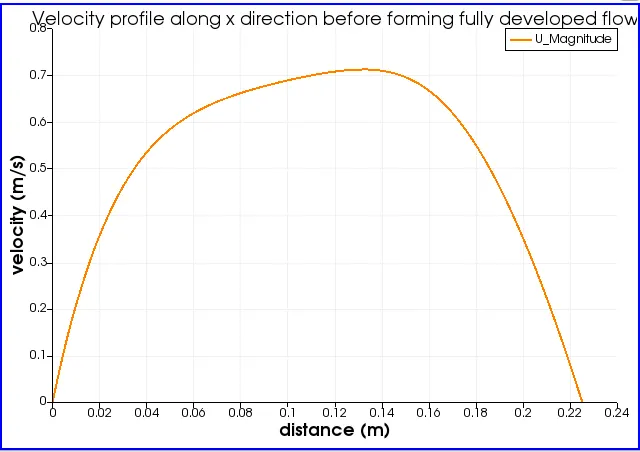
a) At length < hydrodynamic length
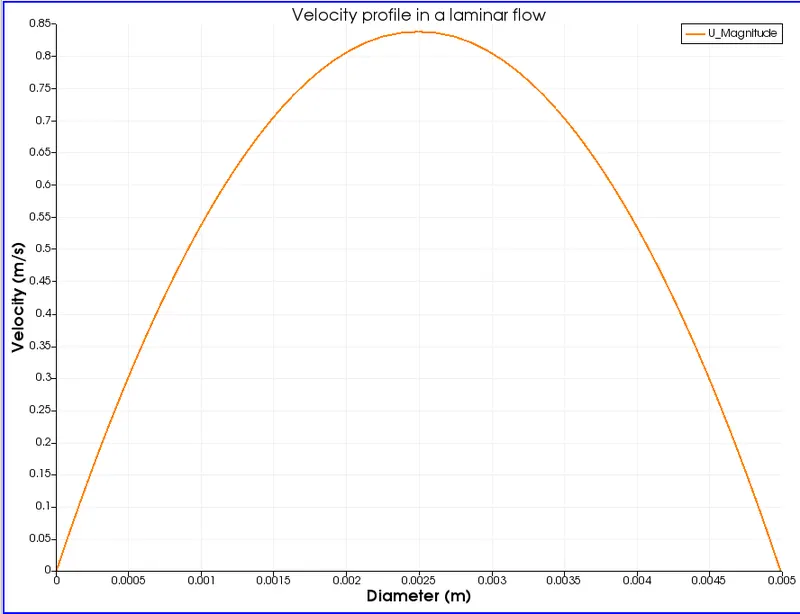
b) At length > hydrodynamic length
2)Pressure drop across length for mesurements after hydrodynamic length was also obtained .
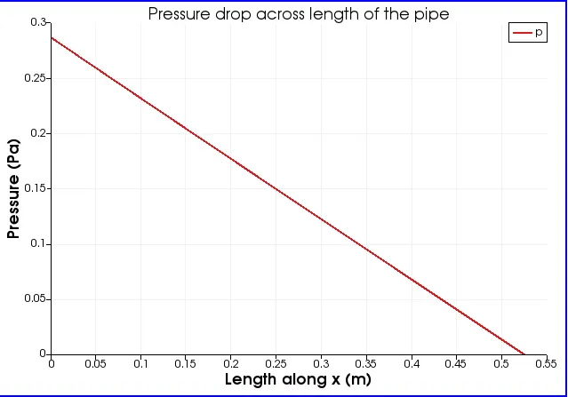
`trianglep` from graph = .28
`trianglep_(actual) = trianglep *rho`
here we take water as working fluid .
hence we get `trianglep = 0.28*10^3`=280 n/m^2
`trianglep_(analytical) = (32.mu.L.V_(avg))/ D^2`
where L = Total length of pipe - Hydrodynamic length of pipe . =1.05 - 0.525=0.525
`mu` = 1.0016e-3
`V_(avg) = (Re*nu)/D` = 2100x1.0034e-6 / .005 = 0.42 m/s
substituting all these values in above equation
`triangle p = (32*1.0016*10^-3*0.525*0.42)/ .005^2` = 282.69 n/m^2
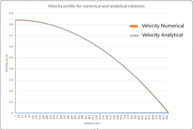
3) To compare velocity profile of numerical and analytical solution .
4)
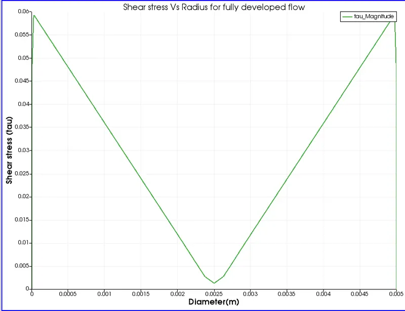
To plot shear stress for fully developed flow
Results :
1) We can observe from first two velocity graphs that the velocity profile obtianed for calculated hydrodynamic length hold true , since it is only for graphs plotted for length > 0.525 m , we get a parabolic profile .
2) The plots from output case 3 shows that the values for analytical and numerical solutions are very close . Hence we can asssume that our numerical calculations hold accurate .
3)
Max velocity
From the plot , we get Umax = 0.84
from calculated value, Vavg= 0.42
Hence the equation`U_(max) = 2V_(avg)` hold good as per our results
Pressure Drop
`trianglep` from graph = .28
`trianglep_(actual) = trianglep *rho`
here we take water as working fluid .
hence we get `trianglep = 0.28*10^3`=280 n/m^2
`trianglep_(analytical) = (32.mu.L.V_(avg))/ D^2`
where L = Total length of pipe - Hydrodynamic length of pipe . =1.05 - 0.525=0.525
`mu` = 1.0016e-3
`V_(avg) = (Re*nu)/D` = 2100x1.0034e-6 / .005 = 0.42 m/s
substituting all these values in above equation
`triangle p = (32*1.0016*10^-3*0.525*0.42)/ .005^2` = 282.69 n/m^2
4)
From the graph in case 4 , we can observe that the maximum shear stress in formed near the walls . We can observe that the shear stress decreases towars the centre of the pipe , and is minimum at the centre of the pipe .