Emission characterization and comparison between Open-W and Re-entrant Omega Bowl shape on a CAT3410 engine.
Emission Characterization on a CAT3410 engine
In this project, the simulation of two different bowl profiles piston geometries of engine(open-w and omega) types has been analyzed. Useful performance parameters are studied and animations show different plots were constructed. Characterization of NOx, soot, and UHC emissions was modeled using suitable models.
----------------------------------------------------------------------------------------------------------------------------
Diesel Engine
The diesel engine is an internal-combustion engine in which air is compressed to a sufficiently high temperature to ignite diesel fuel injected into the cylinder, where combustion and expansion actuate a piston. It converts the chemical energy stored in the fuel into mechanical energy, which can be used to power freight trucks, large tractors, locomotives, and marine vessels. A limited number of automobiles also are diesel-powered, as are some electric-power generator sets.
 |
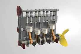 |
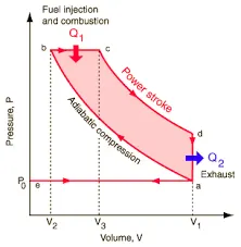
The diesel engine is an intermittent-combustion piston-cylinder device. It operates on either a two-stroke or four-stroke cycle (see figure); however, unlike the spark-ignition gasoline engine, the diesel engine induces only air into the combustion chamber on its intake stroke. Diesel engines are typically constructed with compression ratios in the range of 14:1 to 22:1. Both two-stroke and four-stroke engine designs can be found among engines with bores (cylinder diameters) less than 600 mm (24 inches). Engines with bores of greater than 600 mm are almost exclusively two-stroke cycle systems.
The diesel engine gains its energy by burning fuel injected or sprayed into the compressed, hot air charge within the cylinder. The air must be heated to a temperature greater than the temperature at which the injected fuel can ignite. Fuel sprayed into air that has a temperature higher than the “auto-ignition” temperature of the fuel spontaneously reacts with the oxygen in the air and burns. Air temperatures are typically more than 526 °C (979 °F); however, at engine start-up, supplemental heating of the cylinders is sometimes employed, since the temperature of the air within the cylinders is determined by both the engine’s compression ratio and its current operating temperature. Diesel engines are sometimes called compression-ignition engines because initiation of combustion relies on air heated by compression rather than on an electric spark.
In a diesel engine, fuel is introduced as the piston approaches the top dead center of its stroke. The fuel is introduced under high pressure either into a precombustion chamber or directly into the piston-cylinder combustion chamber. Except for small, high-speed systems, diesel engines use direct injection.
Diesel engine fuel-injection systems are typically designed to provide injection pressures in the range of 7 to 70 megapascals (1,000 to 10,000 pounds per square inch). There are, however, a few higher-pressure systems.
Precise control of fuel injection is critical to the performance of a diesel engine. Since the entire combustion process is controlled by fuel injection, injection must begin at the correct piston position (i.e., crank angle). At first, the fuel is burned in a nearly constant-volume process while the piston is near the top dead center. As the piston moves away from this position, fuel injection is continued, and the combustion process then appears as a nearly constant-pressure process.
The combustion process in a diesel engine is heterogeneous—that is, the fuel and air are not premixed before the initiation of combustion. Consequently, rapid vaporization and mixing of fuel in the air are very important for the thorough burning of the injected fuel. This places much emphasis on injector nozzle design, especially in direct-injection engines.
Engine work is obtained during the power stroke. The power stroke includes both the constant-pressure process during combustion and the expansion of the hot products of combustion after fuel injection ceases.
Diesel engines are often turbocharged and aftercooled. The addition of a turbocharger and an aftercooler can enhance the performance of a diesel engine in terms of both power and efficiency.
The most outstanding feature of the diesel engine is its efficiency. By compressing air rather than using an air-fuel mixture, the diesel engine is not limited by the preignition problems that plague high-compression spark-ignition engines. Thus, higher compression ratios can be achieved with diesel engines than with the spark-ignition variety; commensurately, higher theoretical cycle efficiencies, when compared with the latter, can often be realized. It should be noted that for a given compression ratio the theoretical efficiency of the spark-ignition engine is greater than that of the compression-ignition engine; however, in practice, it is possible to operate compression-ignition engines at compression ratios high enough to produce efficiencies greater than those attainable with spark-ignition systems. Furthermore, diesel engines do not rely on throttling the intake mixture to control power. As such, the idling and reduced-power efficiency of the diesel is far superior to that of the spark-ignition engine.
The principal drawback of diesel engines is their emission of air pollutants. These engines typically discharge high levels of particulate matter (soot), reactive nitrogen compounds (commonly designated NOx), and odor compared with spark-ignition engines. Consequently, in the small-engine category, consumer acceptance is low.
A diesel engine is started by driving it from some external power source until conditions have been established under which the engine can run by its power. The simplest starting method is to admit air from a high-pressure source—about 1.7 to nearly 2.4 megapascals—to each of the cylinders in turn on their normal firing stroke. The compressed air becomes heated sufficiently to ignite the fuel. Other starting methods involve auxiliary equipment and include admitting blasts of compressed air to an air-activated motor geared to rotate a large engine’s flywheel; supplying electric current to an electric starting motor, similarly geared to the engine flywheel; and applying a small gasoline engine geared to the engine flywheel. The selection of the most suitable starting method depends on the physical size of the engine to be started, the nature of the connected load, and whether or not the load can be disconnected during starting.
----------------------------------------------------------------------------------------------------------------------------
Spray modeling
Converge has built-in models utilized for spray processes including liquid atomization, drop breakup, collision, coalescence, turbulent dispersion, and drop evaporation. These models have mathematical approximations necessary to capture the physics behind the processes mentioned above and the combustion aspect as well.
In IC engines, the fuel is sprayed in the combustion chamber or near intake valves. This fuel spray can be completely simulated using CFD multiphase simulations, but doing so in an IC engine simulation would result in the simulation running for very long. This can be prevented if we statistically model the same effect of the spray instead of simulating it. This approximating process of fuel sprays is called Spray modeling. Any fuel spray undergoes a mechanism that has the following processes:
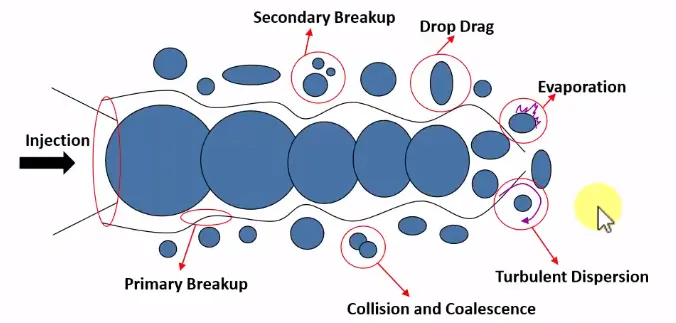
1) Primary Breakup: Splitting of a drop from the mainstream
2) Secondary Breakup: Splitting of a primary drop into multiple drops
3) Drop Drag: Drag caused by air on the moving drop.
4) Collision and coalescence: Collision of two or more drops and formation of the new drop.
5) Turbulent dispersion: Transport of mass, heat, or momentum within a system due to random and chaotic time-dependent motions
6) Evaporation: Evaporation of small liquid drops into vapor
The sequence of processes is easy to understand. The mainstream breaks into multiple drops by primary and secondary breakups. New drops are formed due to coalescence. The evaporation reduces the drops and dispersion spreads the drops into the region. While modeling the spray, each process is represented mathematically by using some pre-established models. These create the effect of spray without actually simulating the spray.
To calculate the spray in a simulation, CONVERGE introduces drop parcels into the domain at the injector location at a user-specified rate. Parcels represent a group of identical drops (i.e., same radius, velocity, temperature, etc.) and are used to statistically represent the entire spray field.
Evaporation: The evaporation is simulated using the Frossling or Chiang model. They are responsible for flagging a parcel drop as evaporated or not. They consider the size of the drop and its evaporation properties to make decisions for drops.
Penetration: The fuel spray penetration is also recorded in the software. It calculates this based on how long did the fuel traveled as a liquid. The cell up to which the 0.95*(mass of liquid fuel sprayed) is seen is called the liquid penetration length.
Collision: The software contains two models: the O'Rourke model and the NTC model. These models simulate the collision using a collision grid. Using a collision grid creates accurate particle movement data.
Drop Drag: This is simulated using the Spherical drop drag model or Dynamic drop drag model. The Spherical model calculates the drag coefficient based on assuming the shape of the drop as the sphere, while the dynamic model accounts for variations in drop shape. It uses the TAB model to determine the drop distortion.
Drop wall interaction: When a drop parcel would collide with the wall, it could rebound back, escape or remain on the wall, creating a film. These effects are modeled using: the O'Rourke model or the Kuhnke model.
CONVERGE offers two categories of liquid injection mechanisms: injectors and nozzles. An injector is a group of nozzles that have some of the same characteristics. Each injector can have any number of nozzles, each with its hole size, cone angle, position, and orientation.
Injector models: The models used are 'The kelvin-Helmholtz model' and 'The rayleigh-Taylor model'. These models look after the primary and secondary breakup of parcel drops. The calculations are based on 'The kelvin-Helmholtz instability theory' and 'The rayleigh-Taylor instability theory. These theories are used for surface tension instabilities of the drop, which lead to a fluid breakup.
i) General: For solid cone sprays, converge assumes the injection is conical.
- Parcel distribution: Distribute parcels evenly throughout the cone.
- Penetration: Converge writes the liquid and vapor penetration lengths at each output interval, it calculates vapor penetration length for each nozzle.
-
Liquid fuel mass fraction for calculating spray penetration: 0.95
- Liquid penetration length is the distance that encompasses the calculated penetration spray mass. Converge calculates the penetrated spray mass by multiplying the mass fraction by the total liquid mass in the domain.
- Liquid penetration length is not calculated along the spray axis of the nozzle but it is calculated along the injector axis
- Bin size for calculating vapor penetration: 0.001 m
- Providing bin size for calculating the vapor penetration, cell size is at least 2 times smaller than bin size, especially in the location of spray.
- Fuel vapor mass fraction for calculating vapor penetration: 0.001
- Cell, where the vapor is present, have some minimum amount of vapor and that is characterized by "fuel vapor mass fraction for calculating vapor penetration". Its value 0.001 of means that particular cell content of 1e-3 vapor in terms of mass fraction coma anything less than that can be considered as a cell that not containing vapor
Collision/Breakup/Drag:
Collision model: NTC collision
Collision outcomes: Post-collision outcomes
Enable collision mesh
- Collision calculation based upon if the one parcel is going to hit the other parcel or not.
- Parcels are Lagrangian parcels that have their own space and the gas phase has its own space.
- To perform collision calculation we need another mesh that is different from the original mesh provided. This is called the collision mesh
Collision calculations can be highly grid-sensitive when an underresolved fluid-phase mesh is used. To help alleviate this issue, the collision mesh option has been implemented in CONVERGE, based on the concept of a collision mesh proposed by Hou. In a simulation without collision mesh, parcels collide only with parcels in the same grid cell. This can lead to artifacts in the spray since parcels do not collide across cell walls. This can also slow down computational time because there can be many parcels in larger cells. Using a collision mesh can eliminate both of these problems. Simulations with collision mesh can much more accurately represent the spray dispersion by eliminating grid effects.
Using a collision mesh can eliminate both of these problems. Simulations with collision mesh can much more accurately represent the spray dispersion by eliminating grid effects.
An alternative to the O’Rourke numerical collision scheme is the No Time Counter (NTC) method of Schmidt and Rutland. The NTC method is based on techniques used in gas dynamics for Direct Simulation Monte Carlo (DSMC) calculations. This model is faster and more accurate than O’Rourke’s model under certain conditions.
The NTC method involves stochastic (randomly determined) sub-sampling of the parcels within each cell.
This potentially results in much faster collision calculations. Unlike O'Rourke's method, which incurs an additional computational cost that increases with the square of the number of parcels, the NTC method has a linear cost. O'Rourke's method assumes that multiple collisions can occur between parcels and that this process is governed by a Poisson distribution. However, the Poisson distribution is not correct unless collision has no consequences for the parcels. Since collisions change parcels’ velocities, size, and number, the method of repeated sampling used by the NTC method generates more accurate answers (Schmidt and Rutland, 2000). The NTC method is derived, without assumptions, from the basic probability model for stochastic collision. The basic probability model requires that the cell size is sufficiently small such that spatial variations in spray quantities can be neglected. These assumptions are a subset of those required for deriving the O’Rourke collision mode.
----------------------------------------------------------------------------------------------------------------------------
Combustion modeling
Combustion Facilitates the energy transfer in an engine. Several models of combustion are available in Converge. But by experiments and several simulation studies, the SAGE model is preferred for accuracy in results.
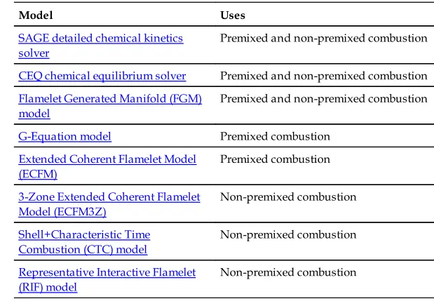
The combustion is modeled by using its reaction mechanism. There are multiple species and intermediate reactions which govern the combustion process. The reaction mechanism of real-life combustion is very large and simulating it directly would take a long time. So, the combustion is solved only for those reactions and species whose presence affects the combustion results. This is called a reduced mechanism file. These all processes of reducing mechanism and solving them is done by various solvers present in the software: SAGE, CTC/ Shell, G-Equation, CEQ, FGM, etc. In this report, the SAGE solver is used, so details of SAGE are only given.
SAGE: It's a detailed chemistry solver which uses local conditions to calculate the reaction rates based on principles of Chemical kinetics. It calculates the heat release, which is used as a source term in fluid flow energy equations. The species are modeled using chemical kinetics ODEs and the values are used in species transport equations. The Solver used to solve the ODEs is CVODES.

Acceleration technique: The SAGE solver is a detailed chemistry solver, meaning that it would calculate values based on the full mechanism instead of reducing it. This takes a lot of time if the calculations are done for every cell in the mesh. So, to increase the speed of solving, the solver is run using a multizone model. All the cells where combustion is going to be solved, are grouped into bins. The bins are created based on the temperature and equivalence ratio of fuel and air. All the cells having the same temperature and equivalence ratio will have the same combustion results. So, the SAGE solver is solved once for each bin, and accordingly, the flow and species data are remapped to the cells. This increases the speed tremendously. The bins can also be created based on multiple variables like pressure, reaction ratio, etc.
PROCEDURE
Geometry Setup
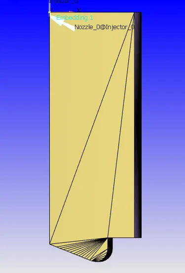
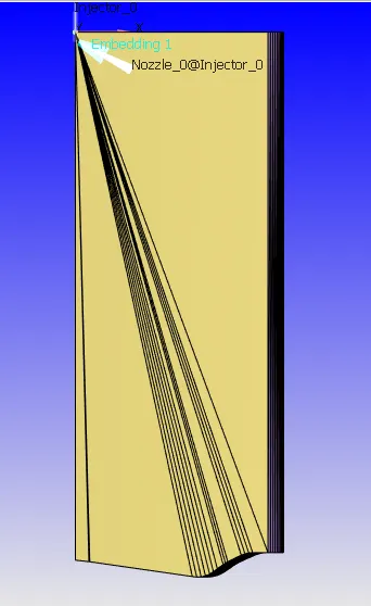
Sector geometry is an extraction of the full 360 deg cylinder into the desired angle. The sectors can be pulled based on the spray-to-angle ratio, for example, if the cylinder has 8 nozzles then 360/8 gives 45 deg. Or if 6 nozzles then 360/6 = 60 deg. This sector will have a single nozzle and will be 1/6th part of the cylinder making this simulation extremely computationally efficient coupled with close cycle analysis.
- The procedure involves first setting up the geometry by making use of the 'Make engine surface sector' tool available under the tools tab.
- Here, we have to set up two different profiles-open v and omega.
- Enter the dimensions of the engine first, as shown in the picture below.
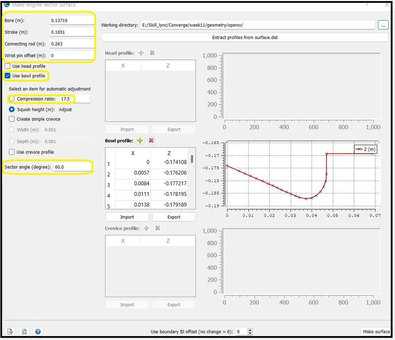
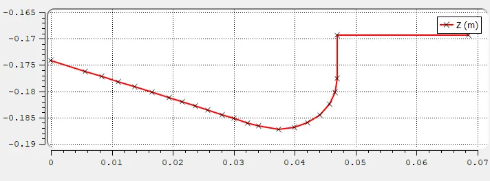
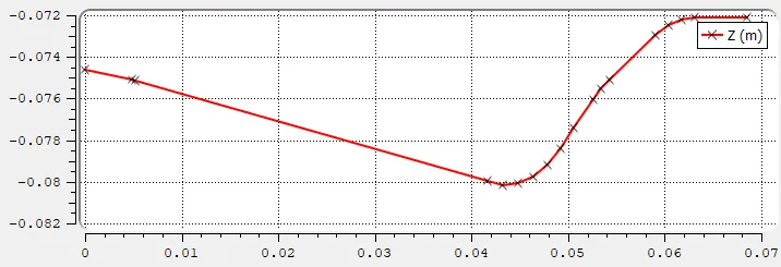
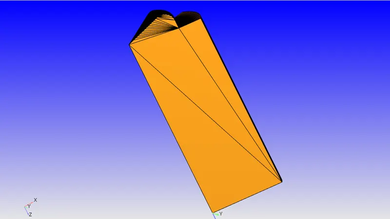
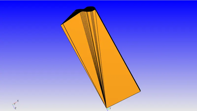
- For the open-v 360 engine, choose extract profile from surface.dat button and enable use bowl profile and import the surface profile for v type and bowl profile for omega type, resulting in two distinct contours as shown below:
Omega Re-entrant Piston Open-W Piston
 |
 |
 |
 |
 |
 |
- V-type
- Click on make surface and the surface is created.
- The next step is to import the necessary input files by going to Files->Import->Import input file(s) and selecting all the .in files and clicking OK.
- The case setup will be automatically set up and the only change that needs to be performed is to go to boundary->piston and choose the type of motion as Piston motion instead of User-defined.
----------------------------------------------------------------------------------------------------------------------------
Application type:- Application type was set to Crank Angle-based IC engine. The values for geometry specifications such as bore dia, rpm, etc were obtained from the Engine Geometric parameters.
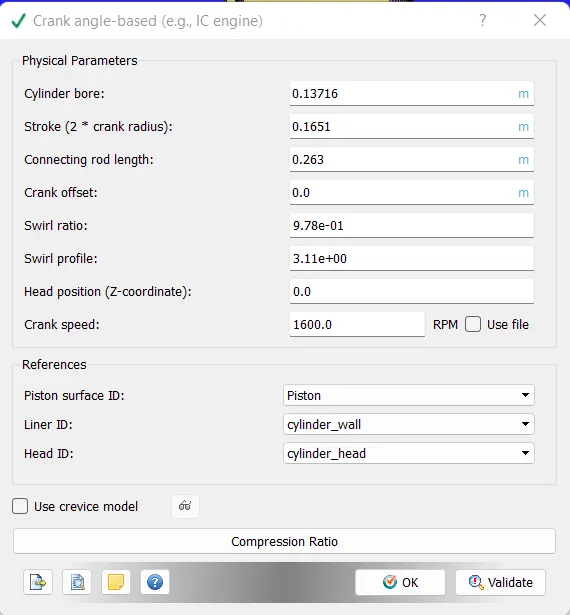
Parcel Simulation- When modeling a simulation that has fuel spray in it, the fuel spray is represented as a Lagrangian Parcel. A lagrangian-based spray model is referred to as a parcel. In this case, set up Diesel2 is the fuel spray.
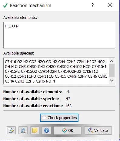
Species: Diesel2 has been added to the 'Parcel'.
Simulation Parameters:
-Run Parameters:- Simulation Mode set to Full Hydrodynamic.
-Solver:- Transient.
-Gas flow Solver:- Compressible.
-Liquid flow Solver:- Incompressible.
Simulation time Parameters:-
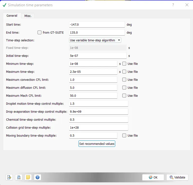
Solver Parameters:
Navier Stokes Solver scheme: PISO
Navier Stokes Solver type: Density-based solver
Numerical values were set as default.
Regions and Events
A region is a collection of boundaries used to differentiate different areas in the boundary. Regions are useful for a variety of reasons
- Used to specify initial conditions by regions
- Control Flow between regions (via events)
- Output results on a region-by-region basis
-Apply grid control techniques by regions
-Map solutions by regions
-Specify combustion models by region
-Determine time step by region-specific CFL numbers.
Events control when the flow is permissible between regions.
In this setup, four regions have been set up, namely the Cylinder region, Intake 1, Intake 2, and Exhaust regions.
Cylinder region
- Temperature - 1360 K (Value provided in the question)
- Pressure-185731 Pa (Value provided in the question)
- Computation of Species mass concentration:- It is assumed that stoichiometric combustion of 'C_7H_16' takes place in the combustion chamber
`C_7H_16+11(O_2+3.76N_2) = 7CO_2+8H_2O+41.36N_2`
For this analysis, it was assumed that the fuel-air mixture is lean as in there is excess oxygen on the product side. This can be verified with the O2 being present in the exhaust gases.
The component of the ICE engine was classified into the different region as shown below
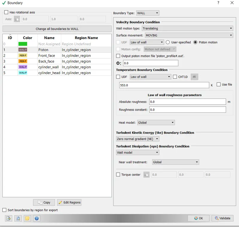
- Piston:- Boundary Type- Wall
Wall Motion Type- Translation
Surface Movement- Moving
----------------------------------------------------------------------------------------------------------------------------
Boundary Conditions:
 |
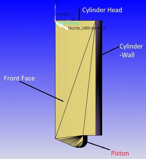 |
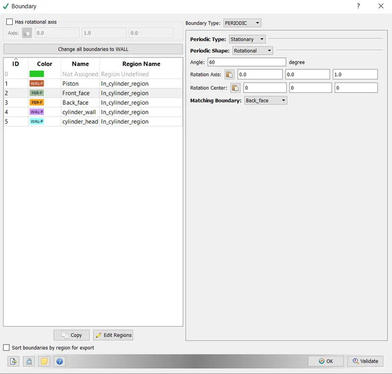
- Front Face
Boundary Type- Periodic
Wall Motion Type- Stationary
Surface Movement- Rotational
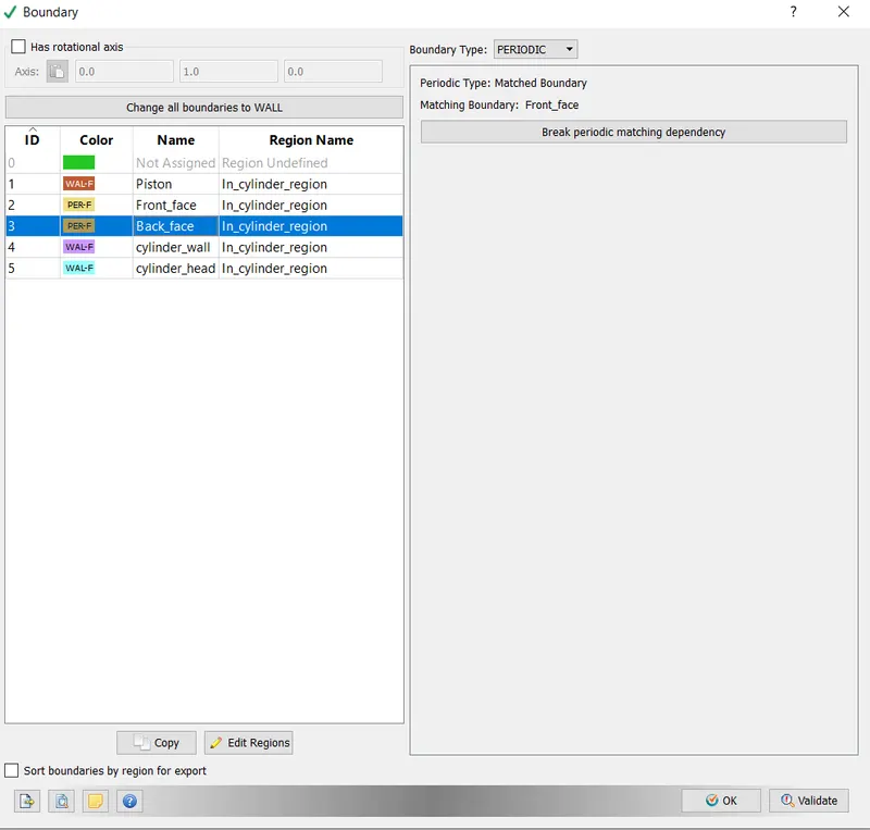
-Back Face:-
Boundary Type- Periodic
Matched Boundary to the front face
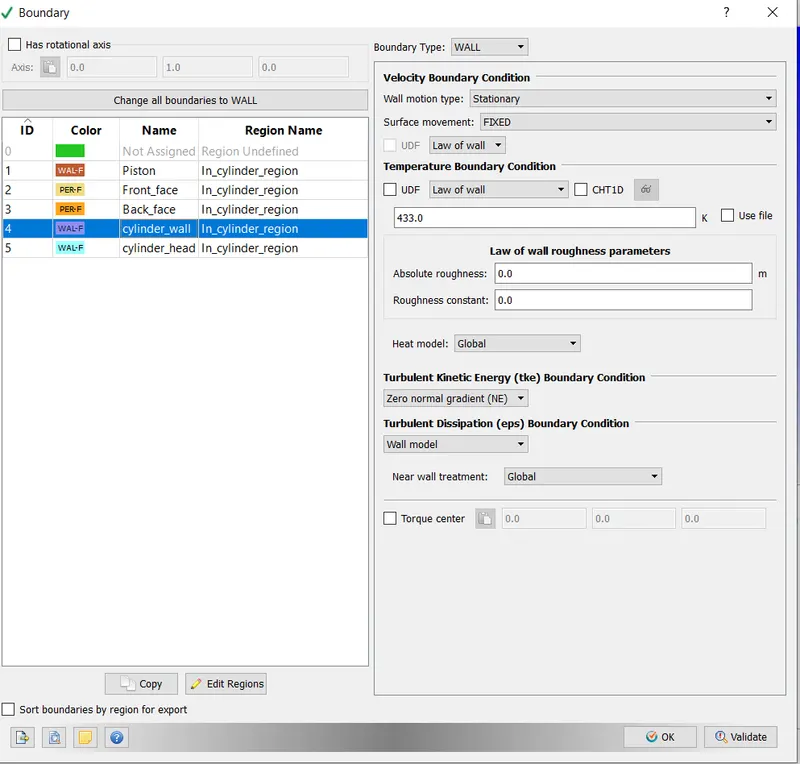
-Cylinder Wall:-
Boundary Type- Wall
Wall Motion Type- Stationary
Surface Movement- Fixed, Law of the Wall
Temperature Boundary Condition- Law of the wall
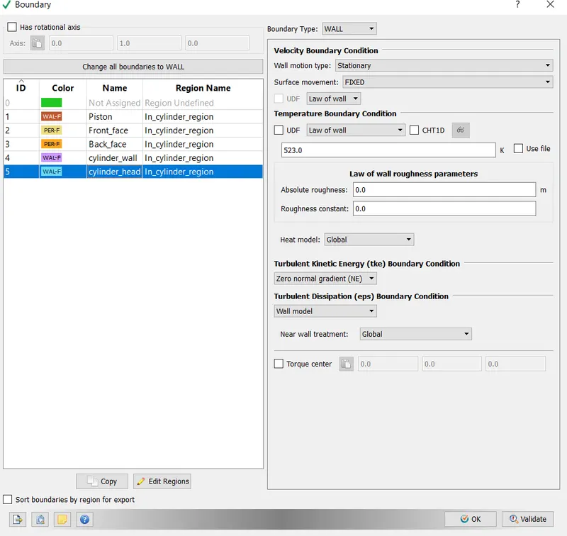
-Cylinder Head:-
Boundary Type- Wall
Wall Motion Type- Stationary
Surface Movement- Fixed
----------------------------------------------------------------------------------------------------------------------------
Physical Modelling
-Spray Modelling:-
Spray modeling is required because solving fluid flow equations describing spray motion directly is not computationally feasible. So a modeling approach is adopted which captures the physics of spray motion.
For liquid sprays, Converge uses a Langrangian solver to model discrete parcels and the Eulerian solver to model the continuous fluid domain. Heat, momentum, and Mass transfer occur between the discrete and continuous phases via source terms in the transport equation.
Converge introduces parcels (collection of drops) into the domain at the injector. Each parcel represents a group of identical drops (same, radius, velocity, temperature). CONVERGE solves for radius, and velocity on a per parcel basis.
Parcel undergoes several Physical processes.
- Primary Breakup
-Secondary Breakup
-Drop Drag
- Collision and coalescence
-Turbulent dispersion
-Evaporation
When fuel is injected, the liquid particles interact with the surrounding air. This interaction causes the creation of drag forces that results in the propagation of disturbances. If the liquid particle is large enough it breaks into smaller particles which then break up into even smaller particles (Primary and secondary breakup). When the smaller secondary particles interact with ambient air, they undergo one or more of the other physical phenomena, namely drop drag, collision, coalescence, Turbulent dispersion, and Evaporation.
For the Full Hydro Case simulation, the following approach was adopted.
- General Setup
i) Parcel Distribution- Distribute Parcels evenly throughout the cone.
ii) Turbulent Dispersion - O Rourke Model (For a gasoline engine, the O Rourke model gives better results).
iii) Evaporation Model enabled.
iv) Frossling model selected.
v) Evaporation source:- Source all base parcel species selected (This implies that IC8H18 (liquid) converted to IC8H18 (gas).
vi) Temperature Discretization enabled.
vii) Radius above which 1 D heat equation will be solved = 1000 m.
viii) No of FV cells per spray parcel =15.
ix) Thermal conductivity- Physical.
-Drop Evaluation
-Film evaporation:- Default value retained.
- Penetration:- Default values.
-Mass Diffusivity:- The default value for Diesel and Kerosene is retained.
-Scaling:- All Values were set to 1.
Collision Break up and modeling
i) Collision model - NTC collision used.
ii) Collision outcomes:- Post-collision outcomes.
iii) Using a collision mesh option that enables.
iv) Drop drag model- Dynamic drop drag.
v) Dynamic drag values set as shown below.
Wall Interaction:-
For Wall Interaction, default values have been retained.
Injector Modeling
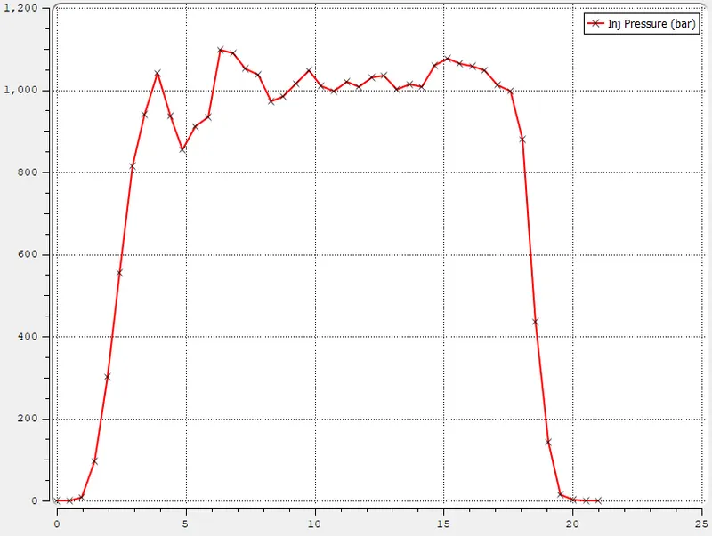
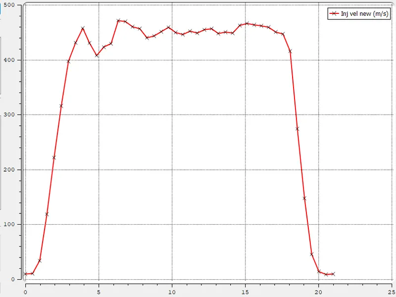
i) Injected Species:- Parcel Species set to C7H16 with mass fraction set to 1.0. The injection rate shape profile was imported.
Models
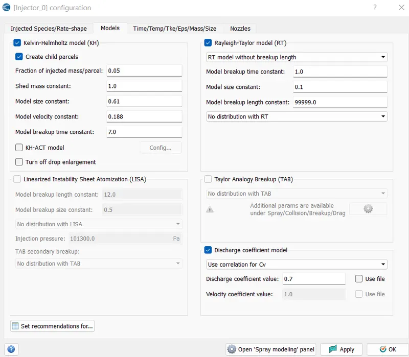
Kelvin- Helmholtz model and Rayleigh- Taylor Model was selected as these are the commonly used models for solid cone sprays. The default constants were retained. The discharge coefficient was set to 0.7.
The default constants control how the breakup of the liquid particles. The stability equation governs the process however do not capture the finer details. The constants govern how long it takes for the breakup and the size of the child droplets.
Injector configuration
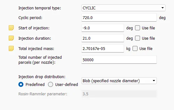
i) Injection temporal type - CYCLIC
ii) Cycle period - 720 degrees
ii) Start of Injection= -9 degree
ii) Injection duration = 21 degree
iii) Total injected mass:- 2.70167 e-05 kg
-Nozzles
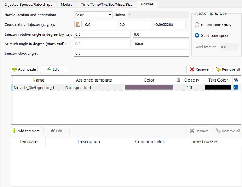
i) Nozzle Location and orientation- Polar.
ii) Injection spray type- Solid cone spray.
ii) Coordinate injectors.
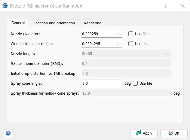
Computation of Maximum Injection pressure:-
Peak Injection Pressure = 1097 (bar)
Peak Injection Velocity New = 471.45 (m/s)
 |
 |
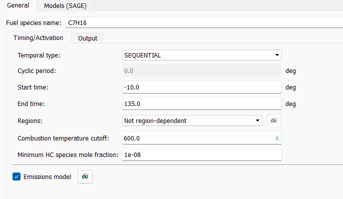
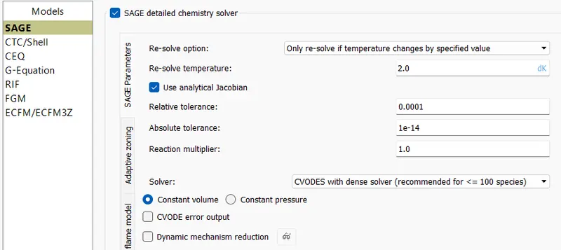
Combustion Modeling:-
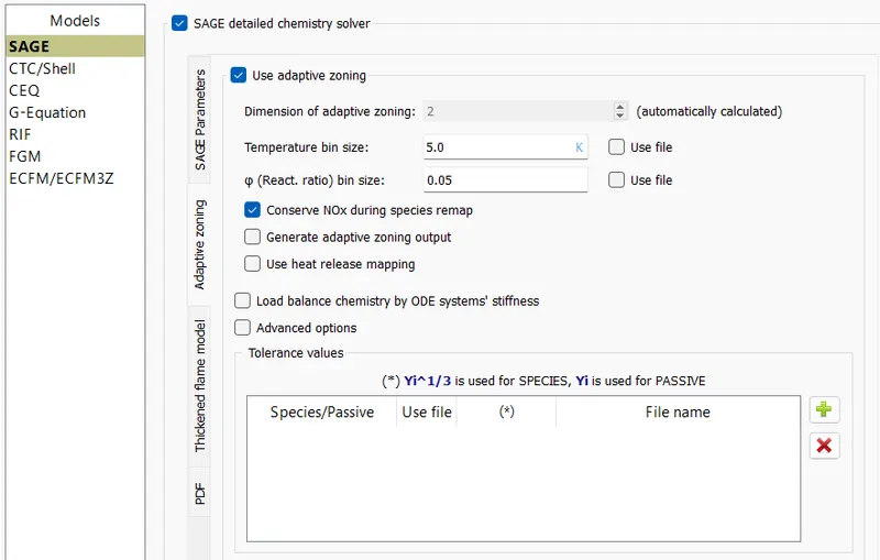
For the simulation, the case was set up as shown below.
The SAGE detailed chemistry solver parameters were set as default.
The combustion was set to start a few crank angles before ignition. The end time for combustion was set considering the opening of the exhaust valve.
Emissions Modeling
- NOx - Thermal NOx model (Extended Zeldovich chosen)
-Hiroyasu NSC soot Model.
----------------------------------------------------------------------------------------------------------------------------
Grid control
CONVERGE uses several tools for controlling grid size during a simulation. Fixed embedding refines a grid at specified locations and times. Grid scaling coarsens or refines the base grid size. Adaptive Mesh Refinement automatically changes the grid based on fluctuating and moving conditions.
- Base grid size was set to 0.004
Adaptive Mesh Refinement
Adaptive mesh refinement increases grid resolution based on curvatures (second derivatives in field variables). It can be permanent or activated at specific times. It is can be activated on a region-by-region basis. It can be activated for both scalar and vector fields.
CONVERGE calculates the Subgrid Scalar (SGS) field as
`ϕ′=ϕ-ϕ¯">ϕ'=ϕ−¯ϕϕ′=ϕ-ϕ¯`
where `phi''= sub grid scalar field
'phi'= actual field
'barphi'= resolved field
CONVERGE uses truncated infinite series to approximate the sub-grid scalar field for any scalar.
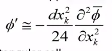
where 'dx_k' is the spacing for a given rectangular cell.
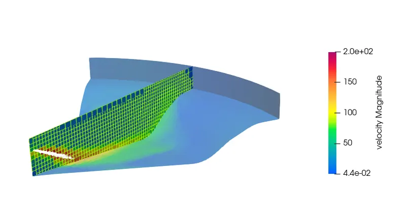
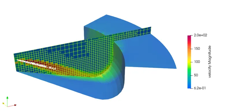
For the full hydro set up two types of AMR is used
1. Velocity
The maximum no of embedding level is 3
SGS criterion is 1m/s
Whenever the curvatures exceed 1m/s, the regions would be automatically refined.
The timing control type is Permanent.
- Temperature.
Max embedding level 3.
SGS criterion 2.5 K.Whenever the curvatures exceed 2.5K, the regions would be automatically refined.
Timing control type- Cyclic
Fixed Embedding
Fixed embedding allows for locally refined mesh in the domain where a finer detail is critical to the accuracy of the solution.
An embedding scale is specified which indicates how CONVERGE will refine the grid in that location
dx_embed= dx_base/(2^(embed scale))
For the Full Hydro setup Fixed embedding was used at the below location
1. Nozzle:-
Entity type- Nozzle
Mode - Sequential
Embed Scale = 2
Grid size at refined locations = `0.004/2^2 =0.001`
2. Exhaust Valve angles
Entity type- Boundary
Boundary ID- Piston
Mode - Sequential
Embed Scale = 1
Grid size at refined locations = `0.004/2^1 =0.002`
3. Cylinder Head
Entity type- Boundary ID
Boundary ID- cylinder head
Mode - Sequential
Embed Scale = 1
Grid size at refined locations = `0.004/2^1=0.002`
----------------------------------------------------------------------------------------------------------------------------
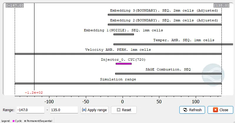
TIMING MAP
Timing map is like a pathway map which lays out all simulation timing details into something like a process chart which displays what procedure is taking place at what degree such as injector function, it displays the type of Grid control parameters are set on it. It gives a handy tool to verify everything in one place & see if some refinement or function is placed as desired or not.
----------------------------------------------------------------------------------------------------------------------------
RESULTS:
Comparison of both bowl profiles (omega re-entrant and open W is done based on Max Pressure, Maximum Temperature, and Emission characteristics.
Total Cells:
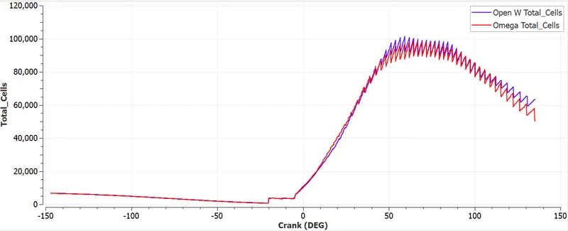
From this figure, comprehension can be drawn that the Open W piston bowl profile used consumed more cells than the Omega piston profile. For Open W total number of cells was 101159 and 96690 for the Omega piston bowl profile.
Pressure variation:
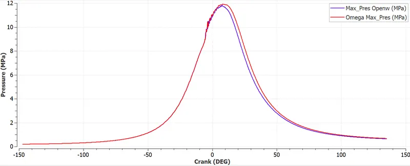
The above graph shows the variation of pressure with the crank angle. Note that the pressure increases until the end of the compression stroke and then decreases gradually after the power stroke. The maximum pressure is observed as 12MPa. By comparison of the two plots carefully, it can be concluded that the maximum pressure rise is achieved in the case of the omega type. A larger pressure rise corresponds to a larger temperature, which in turn causes an increase in combustion efficiency.
Volume variation
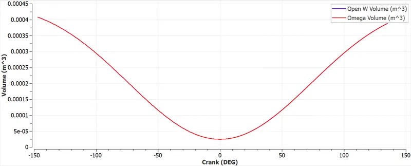
Volume variation along the crank angle. Note that this behavior is exactly the opposite of that observed in the pressure variation. The volume decreases during the compression stroke until the beginning of the power stroke, after which the fuel was added thereby increasing the volume of the fluid inside the chamber. The volume variation for the two different profiles is similar.
Temperature variation
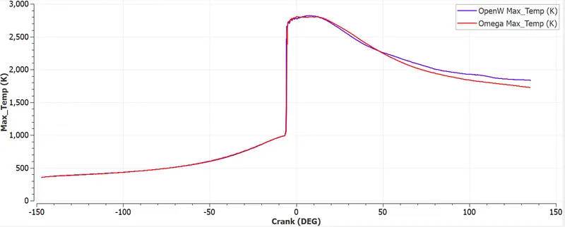
It is noted that the omega piston has a higher temperature when compared to the open w piston. Higher temperature can be attributed to more complete combustion in the cylinder with omega piston when compared to open w piston. The temperature increases steadily throughout the cycle because in the compression stroke, the pressure increases which causes the temperature to increase. In the power stroke, fuel is injected, which causes a further rise in temperature and heat transfer and decreases during the exhaust stroke when the gas is subjected to pushing out of the engine. 2821K for Open W and 2809K for Omega re-entrant.
Heat Release Rate
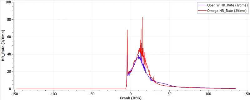
Heat release & Integrated heat release is plotted against crank angle. It gives the Amount of heat i.e total amount of energy released from the combustion process. From the total heat released in the combustion chamber, the combustion efficiency of the engine can be determined. The lower heat release rate in open W indicates some unburnt fuel or delay in burning due to geometrical parameters.
Due to more complete combustion in the cylinder with the omega piston, the magnitude of heat release rate in the piston with this configuration is marginally higher. These sharp peaks and valleys are noise in the data which can be ignored.
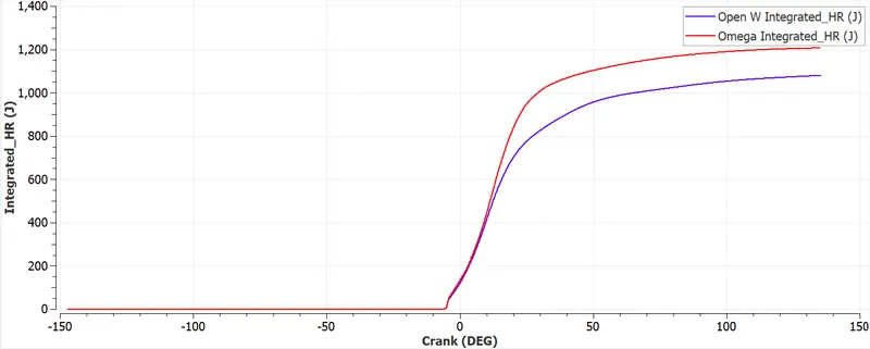
The Integrated Heat Release Rate
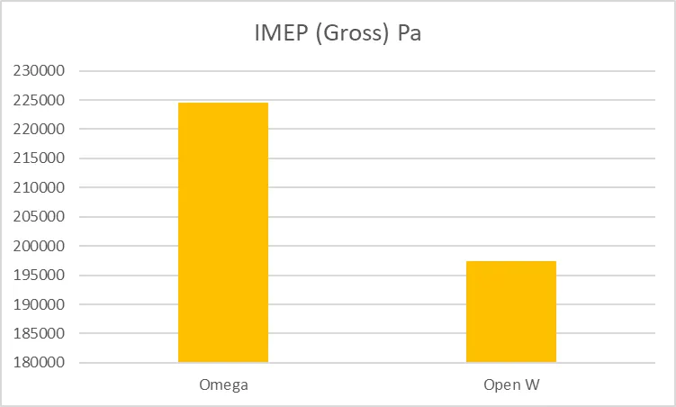
Quantifies the heat that is generated per cycle throughout the volume. For the same reasons as stated above, this value is greater for the piston of omega configuration. OpenW burns a bit slow and a smooth burning curve lower than Omega piston is observed. The omega piston engine burns faster and at a higher release which is advantageous. At the end of the plot, the openW engine ends at a lower release as well. From the engine performance parameters above & Integrated HR data we can determine that the efficiency of the openW piston is lower as compared to Omega.
NOx
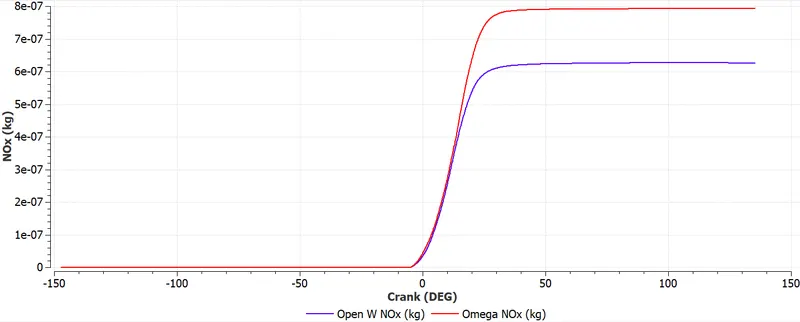
NOx, the cylinder with an omega piston emits more quantity. This is due to the fact that temperatures attained are significantly higher in cylinders with omega pistons. The NOx is significantly higher here than open W. Diesel fuels contain more nitrogen than gasoline and hence they produce higher NOx as compared. This is Zeldovich Nox production. It is low in OpenW however soot is higher, and different tradeoffs compared with engine performance will determine a better design. The critical time period is when burned gas temperatures are at a maximum i.e between the start of combustion and shortly after the occurrence of peak cylinder pressure. The mixture which burns early in the combustion process is especially important since it is compressed to a higher temperature, increasing the NOx formation rate, as combustion proceeds and cylinder pressure increases. And during expansion due to mixing of high and cooler burned gas freezes the NOx chemistry. This effect only occurs in Diesel fuel.
Soot
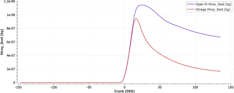
It can be inferred that the combustion in the open_w piston is incomplete. Due to this quantum of by-products such as soot in a cylinder with an open w piston configuration is higher. Soot formation takes place in a diesel combustion environment at temperatures between about 1000 and 2800 K, at pressures of 50 to 100 atm, and with sufficient air overall to burn fully all the fuel. The time available for the formation of solid soot particles from a fraction of fuel is in order of milliseconds. The graph below is the soot formation graph. A large fraction of soot oxidizes within the cylinder before the exhaust process even begins. The soot formed in the OpenW piston is significantly higher than in Omega which is as predicted as there is unburnt fuel at the beginning of combustion in openW and hence is fuel-rich zone at a high temperature.
CO
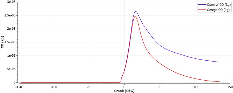
The combustion in the open_w piston is incomplete. Due to this incomplete combustion oxidation of carbon takes place incompletely forming carbon monoxide in place of carbon-di-oxide. There is a 2-3 % difference at peak CO but the very longer degree of dissolution in open-W therefore slightly higher quantity left overall.
UHC (Unburnt Hydro Carbon)
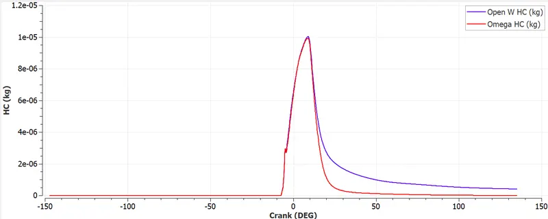
The unburnt Hydro-Carbons result from the Hydro-Carbons present in the fuel escaping from the combustion. The open-W piston does not completely combust the air and fuel mixture because of the lower mean temperature inside the cylinder and also the geometry of the piston affects the process. For the Open-W piston, the UHC is higher when compared to omega pistons. To achieve a good combustion process higher cylinder temperature as well as perfect piston design is essential. Thus we can conclude that the combustion is incomplete in the case of the open-v type.
---------------------------------------------------------------------------------------------------------------------------------
Engine performance calculator
Omega Piston
Open-W Piston
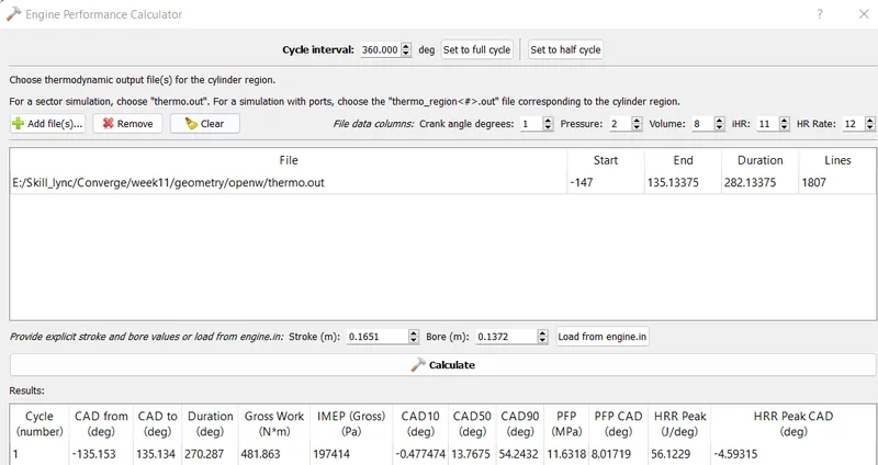
| Open-W Piston | Omega Piston |
|
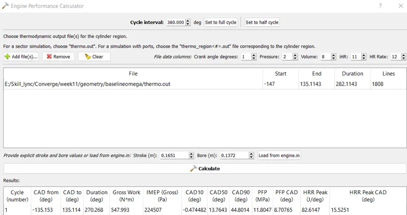
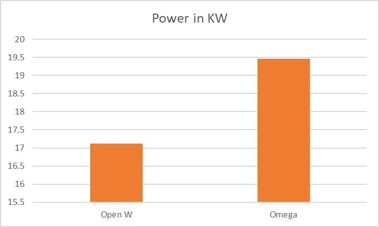
Work done (Gross) = 481.863 Nm Power = Work/Time Time =`270.268^@` RPM - 1600 RPS – 1600/60 = 26.66 RPS DPS – 26.66*360 = 9597.6 Combustion duration in seconds = `270.268/9597.6=0.02815s` Power = Work/Time = 481.863/0.02815 = 17.117 KW. Torque (T) = `60P/(2*pi*N)=60*17117/(2*3.14*1600)=102.2 N.m` |
Work done (Gross) = 547.993 Nm Power = Work/Time Time =`270.287^@` RPM - 1600 RPS – 1600/60 = 26.66 RPS DPS – 26.66*360 = 9597.6 Combustion duration in seconds = `270.287/9597.6=0.02816s` Power = Work/Time = 547.993/0.02816 = 19.4599 KW Torque (T) = `60P/(2*pi*N)=60*19459/(2*3.14*1600)=116.19 N.m` |
 |
 |
----------------------------------------------------------------------------------------------------------------------------
Animations
| Animation Contour | Open-W type bowl design piston. | Omega Re-entrant type piston. |
| Mesh AMR | ||
| Pressure | ||
|
Temperature |
||
| Mass Fraction carbon mono-oxide (CO). | ||
| Mass Fraction NOx. | ||
| Hiroy Soot |
----------------------------------------------------------------------------------------------------------------------------
CONCLUSION
1. Omega piston engine has an edge over OpenW piston engine in this case, there are tradeoffs between both of them but comparatively better one is Omega in terms of Power Production.
2. Engine performance parameters are significantly better in Omega piston engine.
3. Similarly Emissions in Omega design are either low or nearly equivalent to openW in nearly all forms except for NOx, so if primary goal is reducing NOx then OpenW could be preferred. But OpenW design have problems like unburnt fuel during combustion which results in combustion delays and lower peak temperature.
4. Further modification is recommended in case of openW piston, injector angle should be varied which would yeild in better vapourization of fuel spray. Similarly same can be done in Omega to see if more better performance is obtained or faster swirl is obtained.
5. Critical step is to perform the spray & combustion modeling accurately in converge that would route the entire simulation correctly, otherwise the data obtained might not be useful.
6. Grid control parameters like embedding & AMR are critical features in Converge therefore utilized effectively as finer mesh determines the results accuracy & are critical to reduce over all simulation time for extremely detailed cases.
----------------------------------------------------------------------------------------------------------------------------