Week 11 - Louver/Grille characterization

Louver/Grille Characterization

Aim:

To design and evaluate the flow domain comprising a portion of the Hexa grille inside the domain. To study the

parametric method, the parameter trails, and the primary and compound functions to be reported for the

challenge.

Objective:

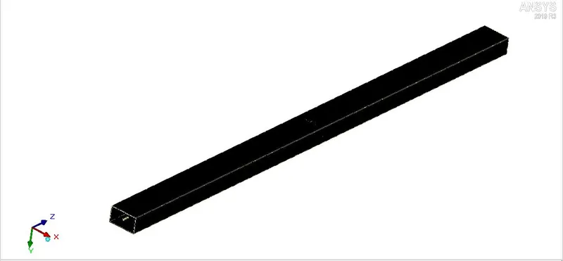
The cabinet has a 160mm in length with the inlet and outlet openings at the ends the cross-sectional area is

(7.363mm x 12.7mm)and the four symmetry walls at the other sides.

The model includes a portion of the Hexa grille placed in streamwise directions at the center of the channel.

The grill has one complete hexagonal hole in the middle and this pattern has been chosen for four

quarters of hexagonal holes located around it as it forms a periodic region which is enough to measure the

loss coefficient.

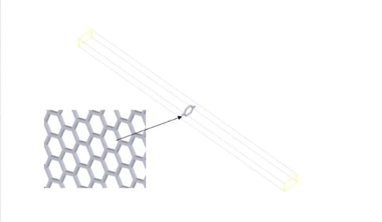
We find only one part of the entire Hexa grille structure into a flow domain from the figure above

Theory:

Simulations of electrical equipment, enclosed electronics components, and electrical systems are typical

applications where grilles are used. The grille loss coefficient is a parameter whose value is a function not just

of the free area ratio, but also of other parameters such as grille design, Reynolds number, grille thickness

and flow regime (laminar or turbulent).

Icepak has an automatic mode that calculates the loss coefficient as a function of the free area ratio. However,

this calculation is based on empirical correlations in the fully turbulent flow regime. Since most applications

are for natural convection in the transitional flow regime it is important to develop a methodology to take into

account the appropriate flow regime.

For more complicated grille design (chevron, louvers, etc.) a wind tunnel simulation is needed to characterize

its pressure loss. Then, it is important to have a methodology to obtain accurate and consistent results.

Geometry:

First, after creating a new project in the icepak, we need to build a cabinet by creating a new project in the

icepak it gives us a cabinet for simulation results. To that cabinet, we need to do the necessary changes as

per our requirements. In our case, the cabinet or flow domain should be 240 mm in length The cabinet height

and width are the same as the Hexa grille we produce.

For the Hexa grille layout, the real measurements are 7.363 mm x 12.7 mm x 1 mm

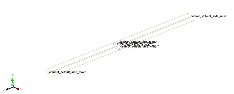
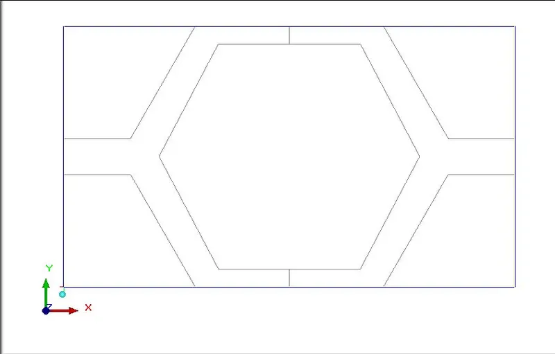
The figure above shows the openings we provided the cabinet and the Hexa grille vertices.

We need to provide the flow with the parametric feature after giving openings and symmetric walls for all four sides of the cabinet.

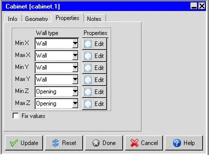
We need to give a parametric function for the flow in the Min-Z direction.

Defining Reynolds number:

Define a velocity parameter at the inlet opening in terms of the Reynolds number Re.

The velocity at the inlet opening in terms of the Reynolds number Re which is customary.

Used in loss coefficient plots in the velocity is calculated as

`Re = (rho*nu*l)/mu`

where Re = Reynolds number

Rho = density of air.

v = Velocity of air.

L or l = Characteristic length.

mu = Dynamic viscosity.

Here L = D_h = 4A/P

D_h = (4*(12.7*7.363)*1e-6)/((2*12.7+2*7.363)*1e-3)

D_h = 0.009321 m

D_h = 9.322e-3 mm.

`Re = (rho*nu*l)/mu = (vl)/nu`

`Re = (vl)/nu`

`l=D_h`

`Re = (v*D_h)/nu`

`(Re*nu)/D_h = v`

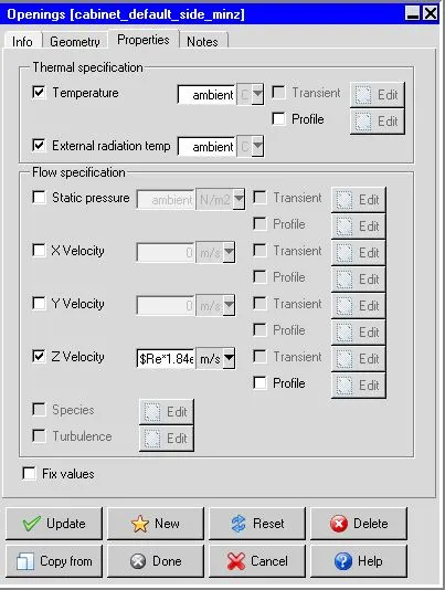
In the cabinet, one of the openings named as the parametric function must be

given Cabinet_default_side_minz in the model manager. Select the Z velocity as we kept the opening in

the Z-direction and set the value to "$Re*1.84e-5/9.322e-3"

Generate mesh:

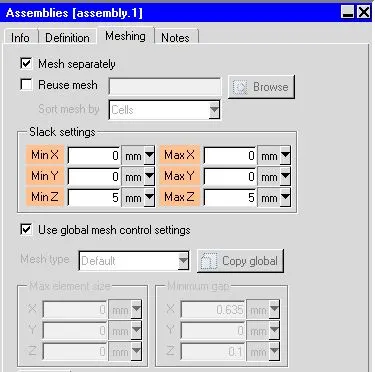
There we produce a separately choice Non-conform mesh for the mesh assemblies. Because we generated

the assembly for the blocks implies we have to assign the z-direction slack values for the single Hexa grille.

Especially in Z-direction for is our interest in finding flow domain is in the Z direction and if we provide X with

the slack values and y-direction the assembly may go outside the cabinet.

So we only give the slack values in the Z direction.

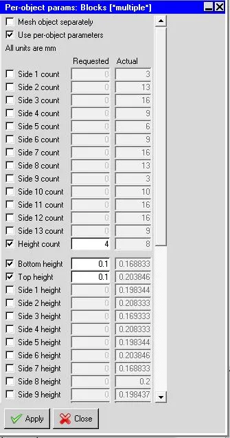
We have also integrated the object parameter values for the even better optimization on the walls of the Hexa

grille.

Now we can create the mesh using the settings in the meshing parameters using mesher HD form with

Normal mesh.

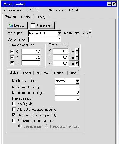
The mesh generates 571496 number of elements and 627347 number of nodes to form an acceptable mesh.

The below figure is the formation of the mesh on the Hexa grill which is the flow direction in the flow domain.

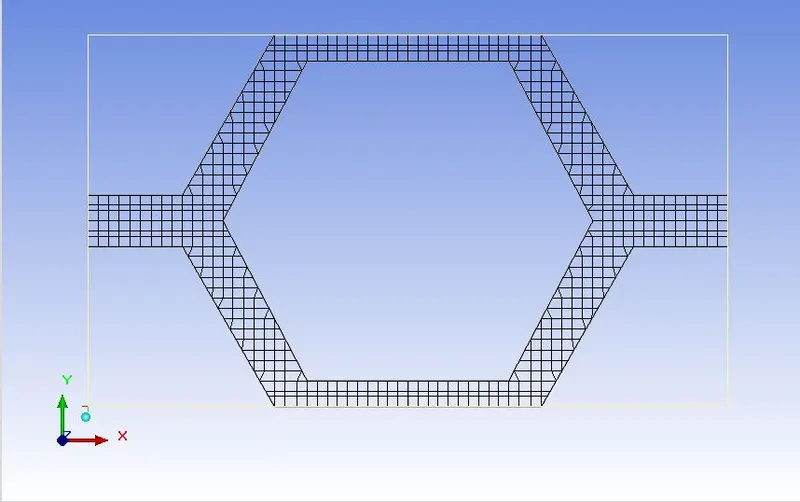
The mesh in the X-direction:

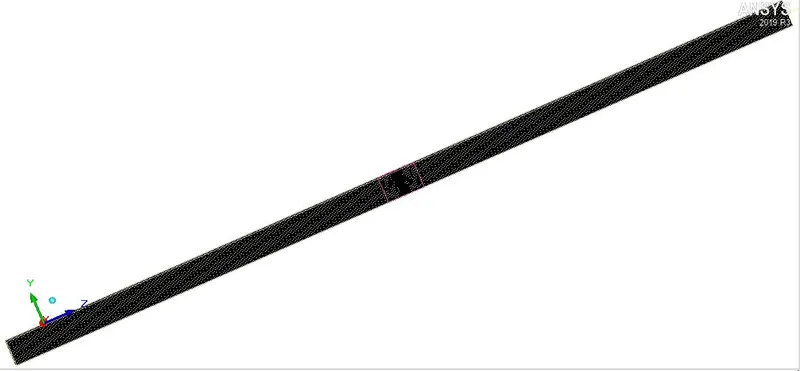
The mesh in the Y-direction:

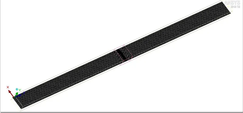
The mesh in the Z-direction:

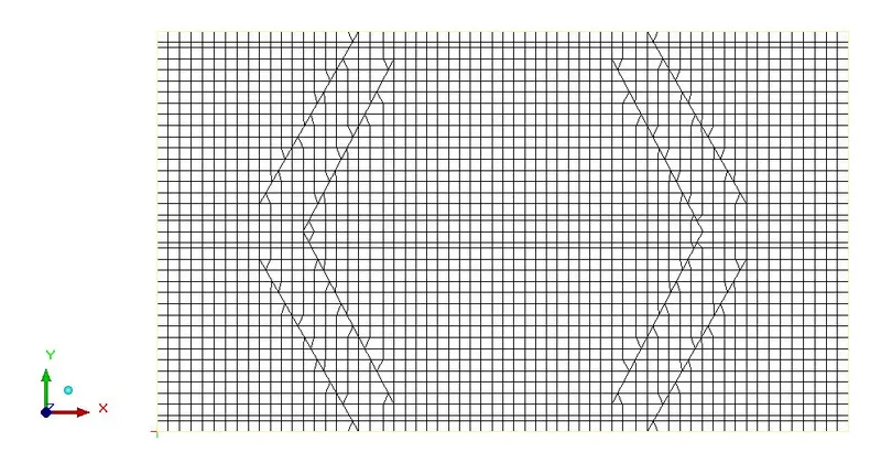
The mesh on the total domain:

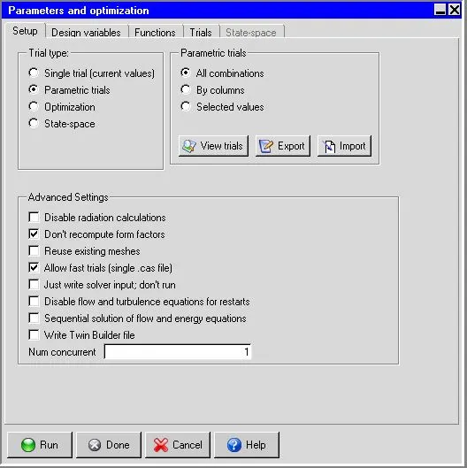
Now we need to give another Eight Reynolds variables in the Run optimization accordingly

• setup
• select parametric trials
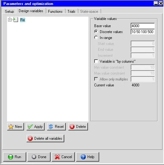
• Design variables
• give the required values in the Discrete values box as "10 50 100 500 1000 2000 3000 4000"

Design variables:

Reynolds number:

Trail Values for the Reynolds number:

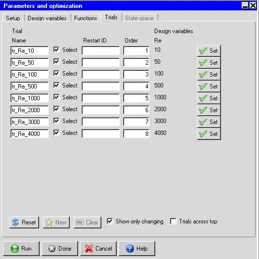
The figure above reflects the total number of trials we will be running in the simulation. This begins with

Reynolds number 10 initially and proceeds to measure all the variables and ends up with the 4000 variables.

Parametric Report that includes pressure and velocities:

First, we need to establish the variables in the summary report for measuring the pressure and velocity that

are also visible in the primary and compound feature domain.

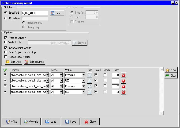
Here we have to include the inputs for the primary functions that we have set up in the overview report

Here in the primary function, we need to create four definitions which are

Static pressure in

Velocity in

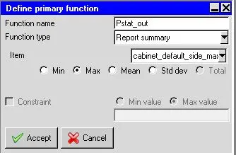
Static pressure out

Velocity out

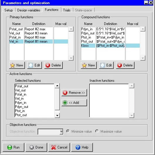
For the compound functions, press the new button the same as the primary function to construct the

definitions.

Here we need to create and find the dynamic pressure inside and out in the compound function. (Pdyn_in,

Pdyn_out) and total in and out pressure (Ptot_in and Ptot_out) and factor k-loss

Now press Done to save and close the parameters and the dialog box for optimization. Click the Run button in

the above to measure or launch the solution after completing the mesh settings.

Setup:

Keep all settings as standard parameters iteration numbers for basic settings, converge conditions, and

advance settings as they are.

Therefore the flow regime will shift from laminar automatically when the numbers of Reynolds are calculated

to turbulence until 2000 when the number of Reynold is calculated for 3000 and 4000.

Residuals:

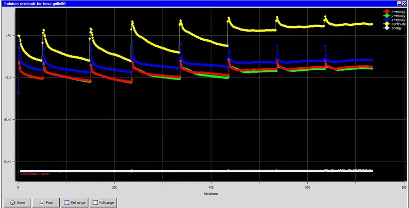
Here the residual plot defines each and every oscillation as the solution for Re 10,50,100 Calculated for other

Reynolds numbers is converged and started.

Results:

The parametric study results for the numbers of Reynolds variables are given in a table. The table includes all

the functions we developed.

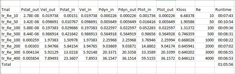
From the above table, we can see clearly that the increase in the number of Reynolds increases the velocity

values and also the strain. The table above is called a summary report of the optimized variables data.

The summary report of the primary functions are:

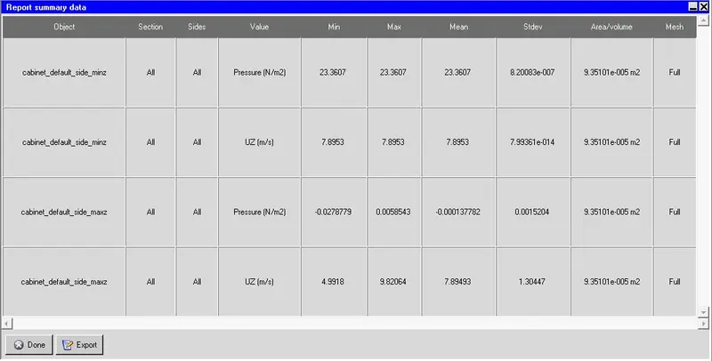
Here in this table, at every Y-opening of the flow domain or cabinet, we can see the max and min velocity and

the pressure.

At the inlet opening the min and maximum velocity is 7.89 m / sec, and the pressure is 23.36 N/m^2.

The min velocity at outlet opening is 4.99 m/sec and max velocity is 9.82 m/sec.

The max pressure at the outlet is almost equal to 0 N/m^2.(actual is 0.0058N/m^2) means

we have a normal or ambient pressure is located in that region.

If we see the pressure there will be a massive drop in the pressure. Any type of obstruction restriction or

roughness in the system will cause resistance to airflow and cause a pressure drop.

The maximum pressure drop from the supply side to the point of use will occur when the compressed air flow

rate and temperature are highest.

K-loss :

The loss coefficient is a dimensionless number (characteristic coefficient) to calculate the heat loss(HL)

`H_L = zeta*(v^2/(2g))`

where

v = characteristic flow velocity in the relevant hydraulic component.

g = Acceleration due to gravity

zeta = loss coefficient

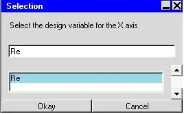
Plot "k-loss" the loss coefficient against the "Re" number in Reynolds Click the plot button in the Parametric

Trials panel to open the selection panel in the selection panel to select Re as the axis variable and click OK.

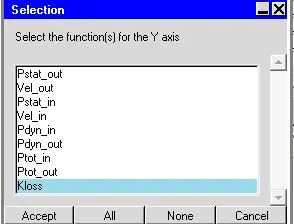
Select k-loss as the y-axis variables and press accept in another selection panel which opens automatically.

Kloss Vs Re:

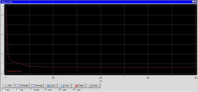
From the above map, we can conclude that the loss coefficient is also decreasing, as the number of Reynolds

increases. The k-loss becomes almost stationary after it enters the turbulence region, which changes at a rate

of 1e-3.

Velocity:

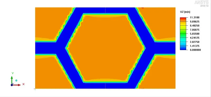
The max velocity recorded inside the flow domain is 11.31 m/sec.

The result illustrates the velocity and flows on the walls of the Hexa grille and the neighboring area.We can see how the velocity from the walls of the Hexa grille to the edges and then in the flow domain region

increases.

LOSS COEFFICIENT OF LOUVER :

The Louver plate is designed to provide ventilation for areas where there is excessive humidity or internal

heat. They are conveniently assembled by cutting the appropriate size and adding the louver plate to the

enclosure.

Problem descriptions :

We need to discuss here the k-loss values obtained from the simulations of the Hexa grille. Here, we must

address the k-loss values obtained from the Hexa grille simulations.

In the previous simulation, we commonly took a single value for the loss coefficient, but in this, we have to

manually load or edit k-loss values.

Geometry :

Click on the current project by opening the icepak, and load the given CAD model into the icepak. The cabinet

dimensions we set are 1200 mm * 500 mm * 1300 mm. Only the structure is installed in this domain.

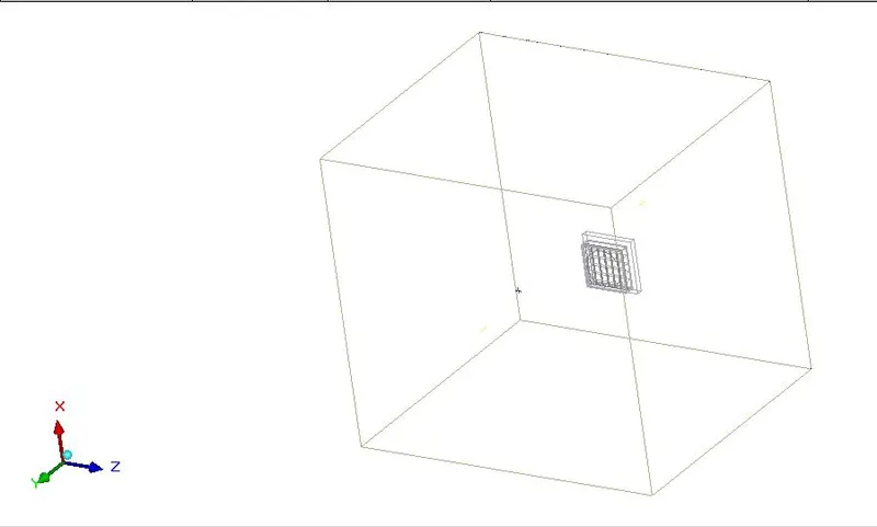
The figure above shows the grilles for the openings and the heat sinks etc. The geometry of the louver is

shown below.

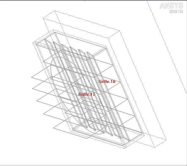
We need to provide the parametric function of the flow after giving the openings and the symmetric walls for

all four sides of the cabinet. We need to give a parametric function for the flow in the Min Y direction.

We need to provide the flow with the parametric feature after giving openings and symmetric walls for all four

sides of the cabinet.

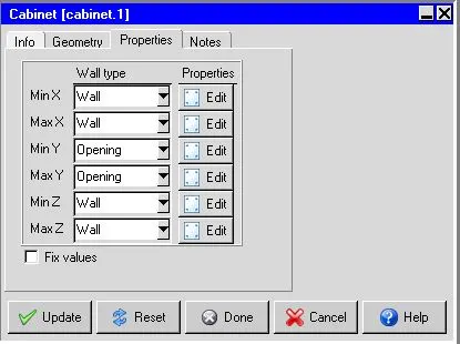
We need to give a parametric function for the flow in the Min-Y direction.

Defining Reynolds number:

Define a velocity parameter at the inlet opening in terms of the Reynolds number Re.

The velocity at the inlet opening in terms of the Reynolds number Re which is customary.Used in loss coefficient plots in the velocity is calculated as

`Re = (rho*nu*l)/mu`

where Re = Reynolds number

Rho = density of air.

v = Velocity of air.

L or l = Characteristic length.

mu = Dynamic viscosity.

Here L = D_h = 4A/P

D_h = (4*(12.7*7.363)*1e-6)/((2*12.7+2*7.363)*1e-3)

D_h = 0.009321 m

D_h = 9.322e-3 mm.

`Re = (rho*nu*l)/mu = (vl)/nu`

`Re = (vl)/nu`

`l=D_h`

`Re = (v*D_h)/nu`

`(Re*nu)/D_h = v`

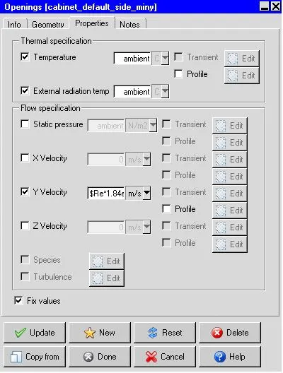
In the cabinet, one of the openings named as the parametric function must be

given Cabinet_default_side_minY in the model manager. Select the Y velocity as we kept the opening in

the Y-direction and set the value to "$Re*1.84e-5/9.322e-3"

Generate mesh:T

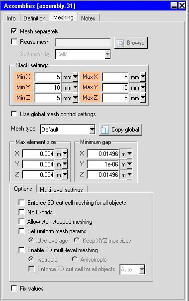
There we produce a separately choice Non-conform mesh for the mesh assemblies. Because we generated

the assembly for the blocks implies we have to assign all direction slack values for the Louver.

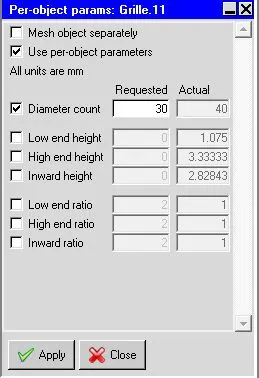
We have also integrated the object parameter values for the even better optimization of the diameter for the

grille.

Now we can create the mesh using the settings in the meshing parameters using mesher HD form with

Normal mesh.

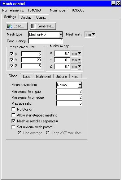
The mesh generates 1040968 number of elements and 1095088 number of nodes to form an acceptable

mesh.

The mesh in the X-direction:

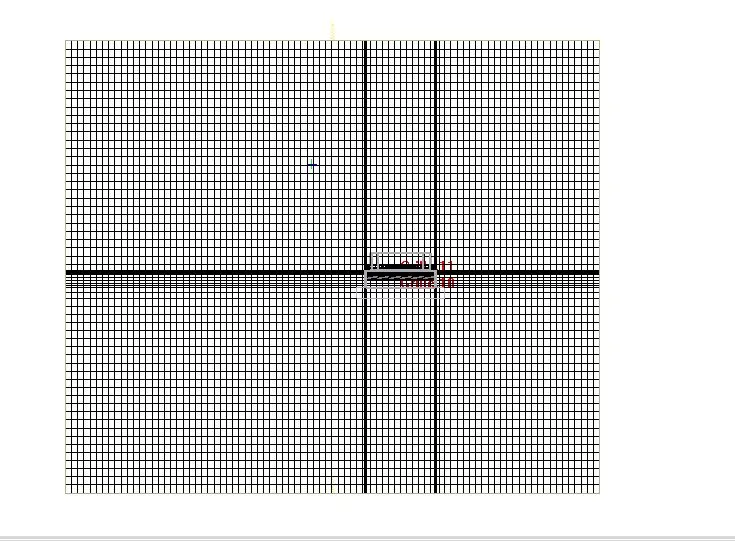
The mesh in the Y-direction:

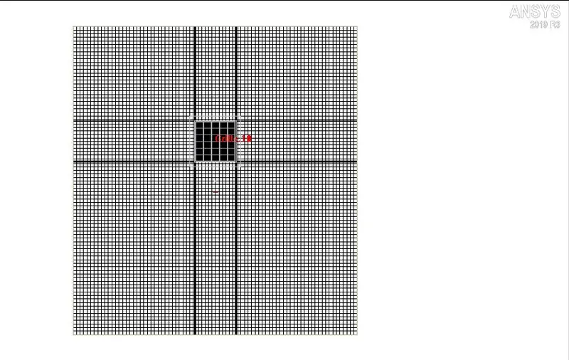
The mesh in the Z-direction:

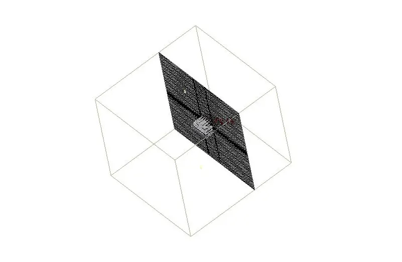
The mesh on the louver domain:

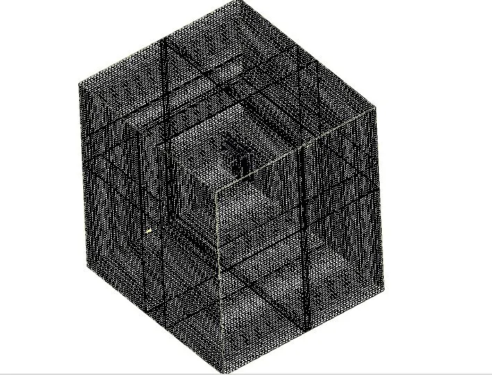
Now we need to give another Eight Reynolds variables in the Run optimization accordingly

• setup
• select parametric trials
• Design variables
• give the required values in the Discrete values box as "10 50 100 500 1000 2000 3000 4000"

Design variables:

Reynolds number:

Trail Values for the Reynolds number:

The figure above reflects the total number of trials we will be running in the simulation. This begins with

Reynolds number 10 initially and proceeds to measure all the variables and ends up with the 4000 variables.

Parametric Report that includes pressure and velocities:

First, we need to establish the variables in the summary report for measuring the pressure and velocity that

are also visible in the primary and compound feature domain.

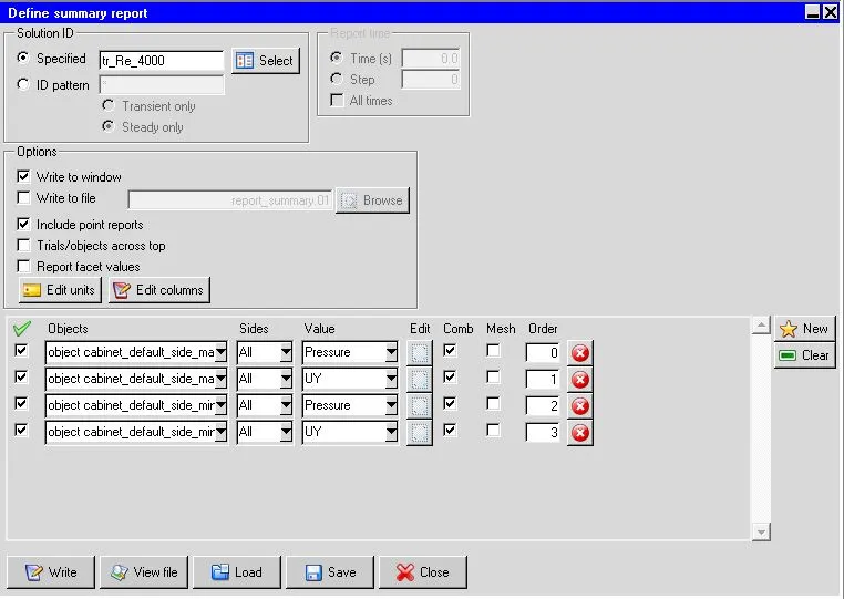
Here we have to include the inputs for the primary functions that we have set up in the overview report

Here in the primary function, we need to create four definitions which are

Static pressure in

Velocity in

Static pressure out

Velocity out

For the compound functions, press the new button the same as the primary function to construct the

definitions.

Here we need to create and find the dynamic pressure inside and out in the compound function. (Pdyn_in,

Pdyn_out) and total in and out pressure (Ptot_in and Ptot_out) and factor k-loss

Now press Done to save and close the parameters and the dialog box for optimization. Click the Run button in

the above to measure or launch the solution after completing the mesh settings.

Setup:

Keep all settings as standard parameters iteration numbers for basic settings, converge conditions, and

advance settings as they are.

Therefore the flow regime will shift from laminar automatically when the numbers of Reynolds are calculated

to turbulence until 2000 when the number of Reynold is calculated for 3000 and 4000.

Residuals:

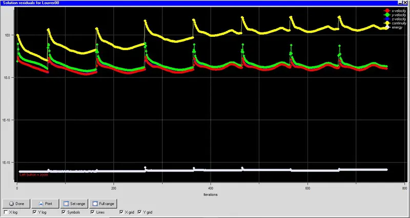
Here the residual plot defines each and every oscillation as the solution for Re 10,50,100 Calculated for other

Reynolds numbers is converged and started.

Results:

The parametric study results for the numbers of Reynolds variables are given in a table. The table includes all

the functions we developed.

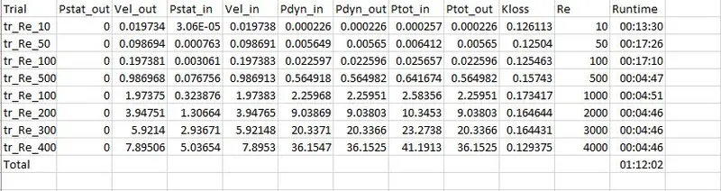
From the above table, we can see clearly that the increase in the number of Reynolds increases the velocity

values and also the strain. The table above is called a summary report of the optimized variables data.

The summary report of the primary functions are:

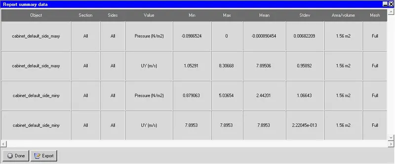
The pressure for the outlet shows the negative and zero because the size of the cabinet is big as compared to

the geometry. At the inlet, the pressure is situated this pressure is developed because of the flow which is

coming into the cabinet

Any type of obstruction in the system will cause resistance to airflow and cause a pressure drop from the

supply side to the points of use that will occur when the compressed air flow rate and temperature are highest.

Loss coefficient K-loss :

The loss coefficient is a dimensionless number (characteristic coefficient) to calculate the heat loss(HL)

`H_L = zeta*(v^2/(2g))`

where

v = characteristic flow velocity in the relevant hydraulic component.

g = Acceleration due to gravity

zeta = loss coefficient

We took a single loss coefficient value in the preceding simulation to determine the criteria for pressure loss.

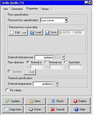
But for now, we're using the loss curve for the requirements on pressure loss.

So that we can define a set of inputs for loss coefficient calculation. The loss curve can be implemented in two

ways we have to had a set of data and the curve of the data. The first approach is by graphics, and the

second method is through the text editor.

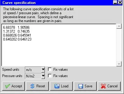
Here we picked the form of the text editor.

A total of 8 values for the 8 different Reynolds number variables as a set we have given.

Plot "k-loss" the loss coefficient against the "Re" number in Reynolds Click the plot button in the Parametric

Trials panel to open the selection panel in the selection panel to select Re as the axis variable and click OK.

Select k-loss as the y-axis variables and press accept in another selection panel which opens automatically.

Kloss Vs Re:

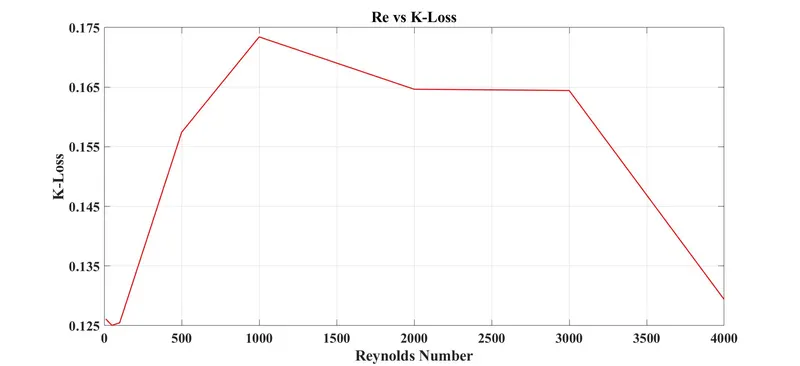
Here if we can see the k_loss it is almost the same with the error of +/-0.1. The highest loss coefficient is

recorded at the Reynolds number 2000 and almost the same for the Reynolds number 3000 with a slight

change.

Velocity Contour:

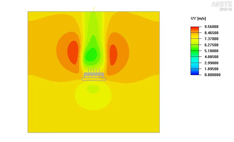
The maximum speed registered within the flow domain is 9.56 m/sec, and the min speed is 0.8m/sec. In the

figure, we can see how speed and flow behave on the louvers walls and in the other region. From the above

diagram, we can see how the flows are separated, and how behind the geometry the wake area is forming.

The velocity animation for the louver has been provided above.

Pressure Contour

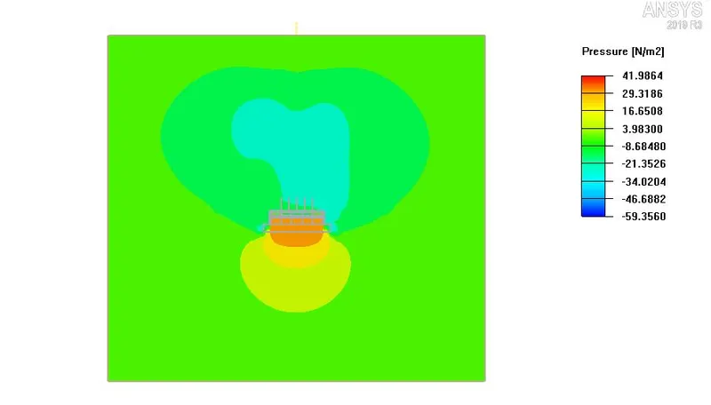
The negative pressure behind the geometry is the principal explanation for the wake region being created.

The peak pressure obtained is on geometry, which implies a natural effect on the components of the

geometry. The max pressure attained in the cabinet is 41.98N/m^2.

Conclusion :

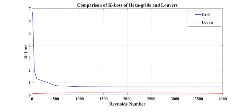
The above graph shows the difference between the Reynolds number Vs k-loss for the Hexa grill and louver.

we can see the difference of the k-loss in between the two grills as the Hexa grill shows the higher loss

coefficient when compared to the louver grill.

From the above graph, we can see the k-loss start with a higher value of the Hexa grill starts from 7 and

reaches a value of 0.6 and the starting highest values of the louver is at 0.17 and ends at a value of 0.12.

We used the parameterization method in this challenge to measure the loss coefficient of a grille and louver

for various Reynolds number(Re) values. We also defined other functions (e.g. at the inlet and outlet static

pressure and velocities) that were reported for various Reynolds numbers. The results show that the loss

coefficient is decreasing as Re rises.

We also learned in the case of the louver how to manually send the loss coefficient values in two forms one is

a text editor and the other is graphical. In this, since the Reynolds number increases the loss coefficient

difference is too small.