week-11 Joint creation and Demonstration

Skill-lync assignment 11

Aim: The objective of this assignment is to demonstrate the various types of joints that can be used in FEA. Spherical, revolute, cylindrical and translational joints are to be modelled for rigid as well as deformable bodies.

Case setup: The following types of joints are to be set up with movement over a time frame of 200 units: -

1. Spherical joint: Allows rotational movement only about 3 axes. Defined by 2 nodes.
2. Revolute joint: Allows rotational movement only about one axis. Defined by 4 nodes.
3. Cylindrical joint: Allows rotational movement about one axis and translational movement along the same axis. Defined by 4 nodes.
4. Translational joint: Allows translational movement only along one direction. Defined by 6 nodes.

The joints are decided to be set up in two separate keyword files. One keyword file will consist of rigid bodies, while the other will consist of deformable bodies.

Procedure: The joints are created through the following series of steps.

1. The LS-PrePost application is launched and the shape mesher tool is used to create two concentric spherical shells at the coordinate (0, 0, 0) and radii of 30 and 35 mm. The top half of the outer shell is deleted to generate two hemispheres. The final geometry is shown below.

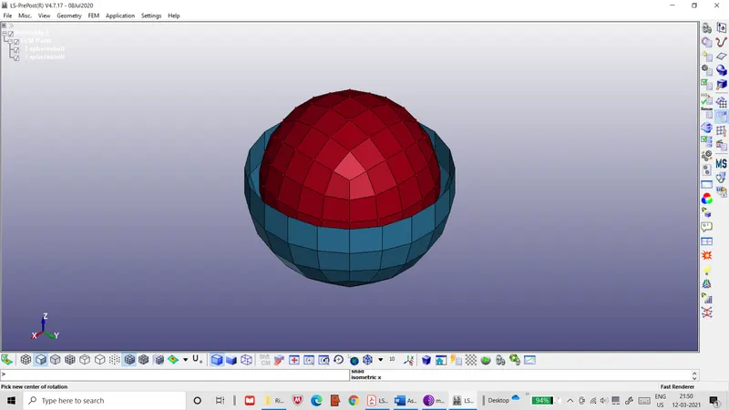Figure 1: Sphere and hemisphere assembly

2. The MAT20 material card with material properties of steel is assigned to the two parts so that they are defined as rigid bodies. A shell section is also defined with a thickness of 1 mm.
3. The inner sphere is fixed in all direction with a BOUNDARY>SPC keyword. The constrained joint is then defined with the concentric centre as both the nodes for its definition. Initial rotational velocities of 0.1 rad/ms about the x, y and z axes are assigned to the outer shell via the INITIAL>VELOCITY_RIGID_BODY keyword.
4. The CONTROL>TERMINATION keyword is included to assign a run time of 40 ms and a time step of 0.01 ms. A constant time step curve is also defined and assigned in order to control time step variation. After checking the model for errors and saving the file, it is then simulated and the resulting animation is observed.
5. In a new keyword file, a pair of rectangular planes 100 mm long and 10 mm wide are created using the shape mesher tool at the coordinates (0, -5, 0) and (0, -5, 5), as shown below.

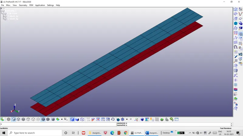Figure 2: Rectangular plane assembly

6. The lower plane is constrained while the revolute joint is defined with the nodes at the centres of these planes as the joint nodes. An initial rotational velocity of 0.1 rad/ms about the z-axis is applied to the upper plane.
7. Step 4 is repeated for this file.
8. The shape mesher tool is used to generate two concentric cylinders with diameters of 30 and 35 mm respectively. An element is deleted from the inner cylinder to create a notch, as shown below.

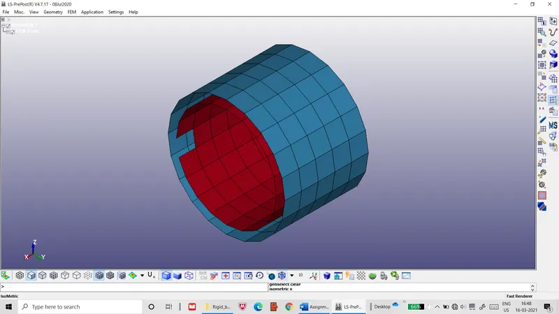Figure 3: Concentric cylinder assembly

9. The outer cylinder is fully constrained and the cylindrical joint is defined with the cylinder ends as joint nodes. An initial translational velocity of 1 mm/ms and a rotational velocity of 1 rad/ms along the x-axis is assigned to the inner cylinder.
10. Step 4 is repeated for this file.
11. The shape mesher tool is used to create two concentric cuboidal (box) shells 100 mm long and with widths of 40 mm and 50 mm respectively. The elements at the ends of the outer box are deleted, as shown below.

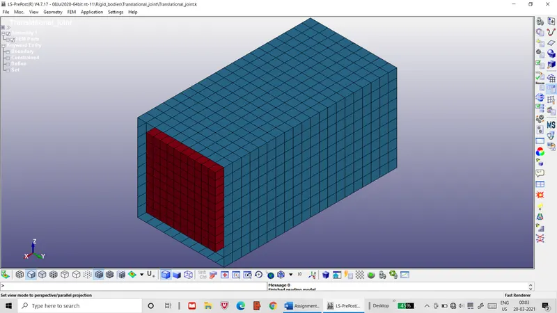Figure 4: Concentric box assembly

12. The outer box is fully constrained and the translational joint is defined with the two ends and a node on the side as joint nodes. An initial translational velocity of 1 mm/ms in the x direction is applied to the inner box.
13. Step 4 is repeated for this file.
14. A copy of the keyword file for the spherical joint is made, where the rigid material is replaced with an elastic material via the MAT001 card.
15. Constrained nodal rigid bodies (CNRBs) are defined for the two shells, as illustrated below, so that their master nodes are located at the concentric centre.

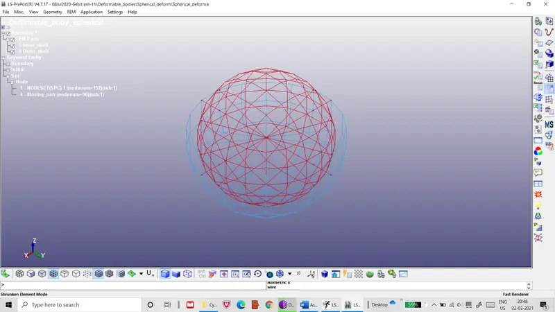Figure 5: CNRBs for spherical joint definition

The master nodes for these CNRBs are used to define a joint between the two. The initial velocity card is replaced with a general velocity card.

16. The file is then saved and run using LS-Run. The resulting animation file is then observed and studied.
17. In a similar manner, a copy of the revolute joint is made and its rigid material is replaced with an elastic material.
18. 4 CNRBs are defined at the centres of the planes, as shown below.

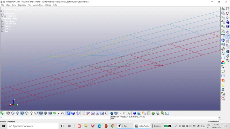Figure 6: CNRBs for revolute joint definition

The master nodes of these CNRBs are used to define the revolute joint.

19. A rotational speed 1 rad/msec about the y axis is assigned to the upper plane.
20. Step 16 is repeated for this file.
21. A copy of the cylindrical joint keyword file is edited and the rigid material is replaced with an elastic material and the rigid body velocity card is replaced by a general velocity card.
22. CNRBs are created at the ends of both the cylinders, as shown below and their master nodes are used to define a cylindrical joint.

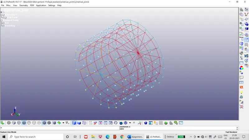Figure 7: CNRBs for cylindrical joint definition

23. Step 16 is repeated.
24. A copy of the translational joint is edited and their material and velocity cards are replaced like in the previous files.
25. CNRBs are created at the ends and the centres of the two boxes, as illustrated below, and their master nodes are used to define a translational joint.

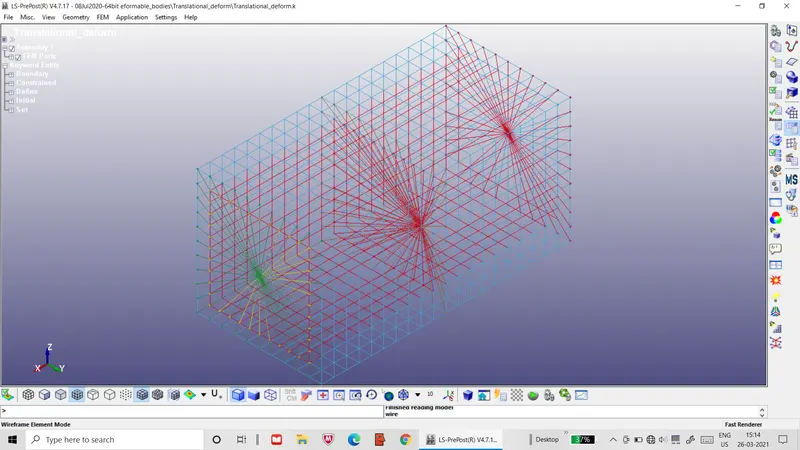Figure 8: CNRBs for translational joint definition

26. Step 16 is repeated.

Results: The following observations are made for the various joint simulations.

• For all the joints, time step control was an essential requirement. Without it, the defined joints do not properly constrain the associated parts.
• For deformable joints, CNRBs had to be carefully defined with proper location of master nodes and correct allocation of CNRBs to each part.
• The CNRBs themselves required proper definition with proper distribution of slave nodes and surrounding elements for their proper functioning.
• In the case of the deformable cylindrical joint, the constraint release flags for both rotational and translational movement had to be set to 0 (rigid body behaviour) for proper simulation.

Conclusion: The various kinds of joints, both rigid and deformable variants, have been successfully demonstrated in multiple iterations. The joints successfully showed movement in the desired directions.