week-11 Joint creation and Demonstration

AIM

The aim of this assignment is to understand how to create joints between two different parts of deformable bodies and between rigid bodies. In this case we will try to understand the creation of four main joints revolute,spherical, translational, and rotational joints.

EXPLANATION

*CONSTRAINED_JOINT keyword is used to create joints between two bodies whether they are rigid bodies or deformable bodies. In this assignment we will model four types of joints which are revolute, spherical, translational and rotational and we will model all these joints separately for rigid bodies and deformable bodies as the procedure is slightly different.

CASE SETUP

CASE 1.1: Revolute joint - deformable bodies

A revolute joint allows for only rotational degree of freedom between two parts about a centerline. An image of a revolute joint is shown below.

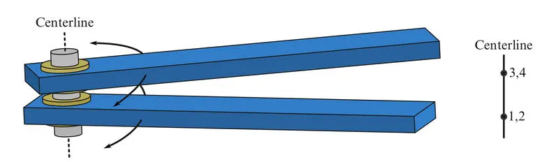
As you can see we need two pairs of coincident nodes to define a revolute joint between two bodies in LS-DYNA. Nodes 1 and 2 are coincident; nodes 3 and 4 are coincident. Nodes 1 and 3 belong to body A; nodes 2 and 4 belong to body B. The relative motion of the two bodies is restricted to rotations about the axis formed by the two pairs of coincident nodes. This axis is labeled the “centerline.”

For demonstrating revolute joint we need two meshed surface. To create this we use the shape mesher tool from the mesh options. Then we select the 4N shell options and input the coordinates of the four corners of our surface and select create. We create two meshed entities so as to demonstrate the joint.

For the creation of our joint we need two pairs of coincident nodes along a centreline, for this, we create them by using node editing option.

*SECTION-SHELL keyword is used to give a shell thickness of 1 mm.

*MAT-ELASTIC is used as the material model with RO = 0.00279, E= 7.31e+04, PR = 0.35.

The nodal pairs along the centreline have to be associated with the bodies to create the joint. For this we use *CONSTRAINED_NODAL RIGID_BODY keyword. In our case nodes 73 and 76 are coincident and nodes 74 and 75 are COINCIDENT. *CONSTRAINED_NODAL_RIGID_BODY keyword is used to associate nodes 73 and 74 to the first body while 76 and 75 are associated with the second body.

* CONSTRAINED_JOINT is used to create the revolute joint between the two bodies. In this card node N1 should belong to body A and node N2 should belong to body B. Also, N1 & N2 should be coincident. Similarly for N3 and N4.

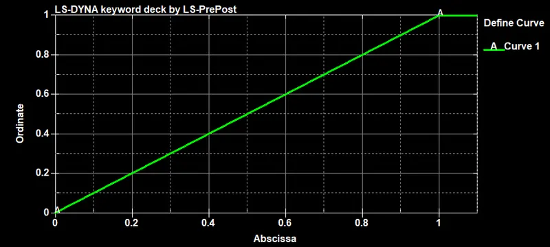
Now, to make this resolute joint work few boundary conditions are essential. So, a displacement along a positive z- direction is applied to one of the nodes on the 2nd Part. The displacement is given using the keyword *BOUNDARY_PRESCRIBED_MOTION_SET. The z-translational degree of freedom is kept free by assigning DOF = 3. For giving the displacement we need to give a load curve. This is done by using the *DEFINE_ CURVE keyword. The displacement curve given,is shown below.

* BOUNDARY_ SPC_SET is used to constrain the nodes of part 1.

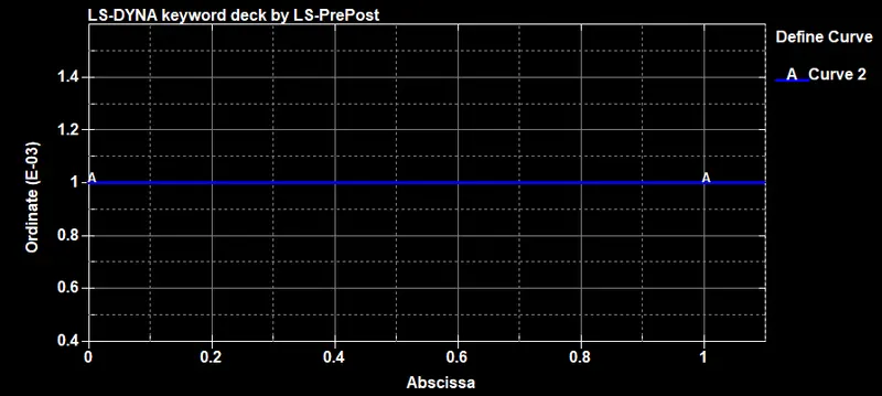
*CONTROL_TIMESTEP card is used and a load curve (Shown below) is assigned using LCTM option. The timestep calculated by the solver for these rigid bodies and this mesh size is large enough and hence for more stability we use smaller timestep for explicit analysis.

* DATABASE_BINARY_D3PLOT is defined to get the result. Also, *DATABASE_ASCII_OPTION is used and the GLSTAT is activated with DT = 0.1.

* CONTROL_TERMINATION is added with termination time being 1ms.

All the parts are assigned with the right material and section using *PART-PART keyword. The simulation is then run to view the working of the joint.

CASE 1.2: Revolute joint -Rigid body.

The revolute joint between two rigid bodies can be made using a similar procedure as above. The only difference here is that we use * CONSTRAINED_ EXTRA_NODES to associate the nodes at the centreline to the two parts. The nodes associated with the 1st part are made into a nodeset, then we associate this nodeset to the 1st part using *CONSTRAINED_EXTRA_NODES_SET.

Also, the one other difference here is that instead of *MAT_ELASTIC material model we use * MAT-RIGID for the two parts.

CASE 2.1: Spherical Joint-deformable body.

This type of joint has all there rotational degrees of freedom. However translational movement is not allowed. Also, only one pair of coincident nodes are required to construct this type of joint. An example of a spherical joint is shown below.

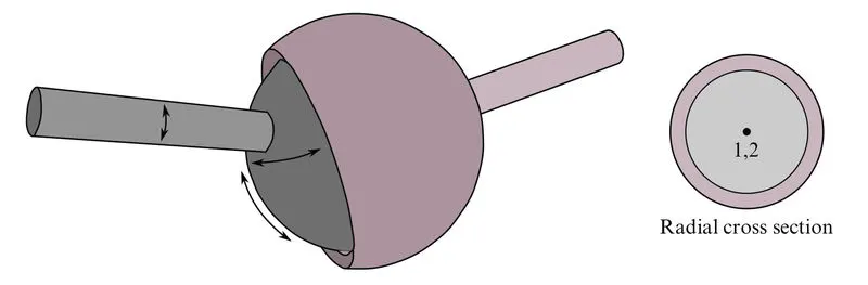
To demonstrate this joint we need two concentric spheres. These spheres can be constructed in the same way as we created the meshed surface earlier using the shape mesher tool. Instead of 4N shell we select sphere shell and give a radius. Here we create two spheres, one larger than the other. Also, using node edit tool we create a pair of coincident nodes at the center. These nodes are associated with the two spheres using *CONSTRAINED_NODAL_RIGID_BODY.

Now, to create the joint ,*CONSTRAINED_JOINT_SPHERICAL keyword is used. Here node N1 belongs to the 1st part and node N2 belongs to the second part.

* BOUNDARY_SPC_SET is used to constrain the nodes of small sphere.BOUNDARY_PRESCRIBED_MOTION-SET is used give rotational movement is x, y and z directions using a loadcurve, similar to the one which was given in the case 1.1. * MAT_ELASTIC is used as the material model with the material same as case 1.1. All other keywords and parameters needed to run the simulation is same as case 1.1. These parameters are input and the simulation is then run.

CASE 2.2: Spherical Joint - Rigid Body

This case is very similar to case 2.1 except that, the two spheres are made rigid body using * MAT_RIGID keyword. The material used in case 1.2 is also used here.

Here the two concentric nodes are associated with the rigid body using *CONSTRAINED_EXTRA_NODES_SET card. All other parameters needed to run the simulation is exactly same as case 2.1.

CASE 3.1: Cylindrical Joint- Deformable body

This joint is derived from the rotational joint by relaxing the constraints along the centreline. This joint admits relative rotation and translation along the centreline.An example of cylindrical joint is shown below.

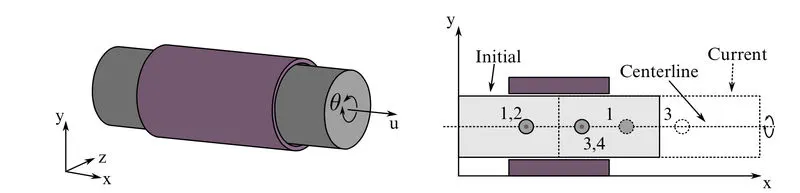
This joint also requires two pairs of coincident nodes along the centreline.

To demonstrate this joint we require two cylinders which are concentric. This can be created by using the shape mesher tool and selecting cylinder shell option. The four extra nodes that we require along the centreline are created using node edit option. The four extra nodes created are associated with the two parts using *CONSTRAINED_NODAL_RIGID_BODY. *MAT-ELASTIC was used as the material model. For joint demonstration the larger cylinder was given a translational motion in x-direction and rotation about x-axis using * CONSTRAINED_MOTION_SET keyword. * SPC_SET was used to fix the small cylinder. All other parameters needed to run the simulation is same as case 1.1

CASE 3.2: Cylindrical Joint-rigid Body

This case closely resembles case 3.1 except that here we use rigid bodies instead of deformable bodies. To change the cylinders to a rigid body we use *MAT-RIGID keyword. To associate the nodes on the centreline to the respective rigid bodies we utilize the keyword *CONSTRAINED_EXTRA_NODE_SET. All other procedure neede to run the simulation is exactly similar to case 3.1.

CASE 4.1: Translational Joint-deformable body.

Translational joint is a cylindrical joint with a third pair of off-centreline nodes which restricts rotation. Aside from translation along the centreline, the two rigid bodies are stuck together.An example of translational joint is shown below.

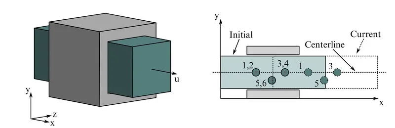
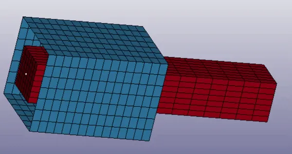
To demostrate this joint we require two box shell. This can be created by using the shape mesher tool and selecting box shell. The elements on the two opposite faces of the large box shell is deleted so that the small shell is inside the large shell box. Here in-addition to the two pairs of coincident nodes along the centreline we need a third pair of coincident nodes which is not on the centreline as is shown on the figure above. These nodes are then associated with the respective bodies using *CONSTRAINED_NODAL_RIGID_BODY. *CONSTRAINED_JOINT_TRANSLATIONAL is used to create the joint. Here N1, N3 and N5 belong to the first part while N2, N4, N6 belong to the second part. *BOUNDARY-PRESCRIBED-MOTION- SET is used to give translational motion along z- direction in this case. The small box shell is fixed using *SPC_SET. All other parameters needed to run this simulation is the same as in case 1.1

CASE 4.2: Translational Joint -Rigid body

In this case the material model that we use is *MAT-RIGID to make the shells a rigid body. Instead of *CONSTRAINED_ RIGID_BODY we use *CONSTRAINED_EXTRA_NODES to associate the extra nodes that we created to the rigid bodies. All other parameters needed to run this simulation is the same as in case 4.1.

RESULT

The simulation of revolute joint of deformable body is shown below.

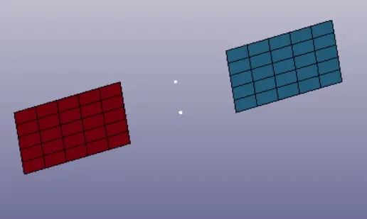
The simulation of revolute joint of rigid body is shown below.

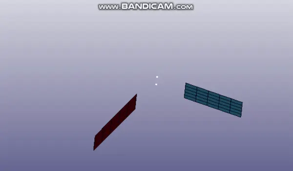
The working of spherical joint for deformable bodies is shown below.

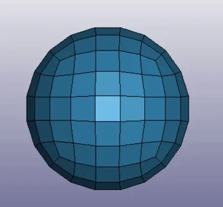
The sectional view of the working of a spherical joint for rigid bodies is shown below.

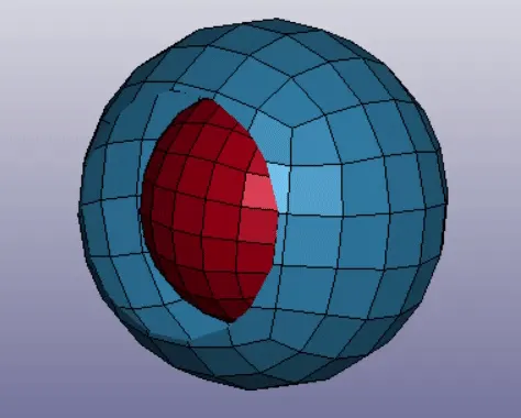
The working of cylindrical joint for deformable bodies is shown below.

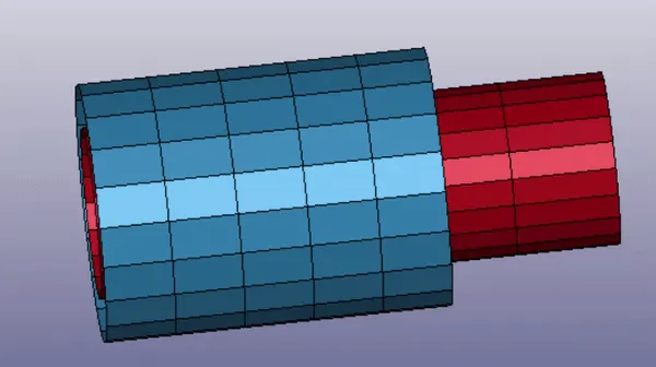
The working of cylindrical joint for rigid bodies is shown below.

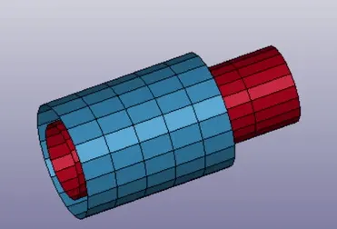
The working of translational joint in deformable bodies is shown below.

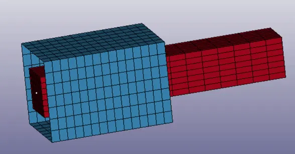
The working of translation joint in deformable bodies is shown below.

CONCLUSION

All the most common and important joints used are studied. The difference in modelling a deformable body joint and rigid body joint is studied.