week-11 Joint creation and Demonstration

Aim:

The aim of the challenge is to lear how to create and model joints in LS_Dyna. The challenge involved creating 4 types of joints between 2 bodies: spherical, revolute, cylindrical and translational joints. Further, each joint had 2 cases: first, between rigid bodies and second, between deformable bodies.

Explanation:

The 4 types of joints in each of the two cases were created using following procedure:

1. Revolute joint

Case 1: Rigid bodies

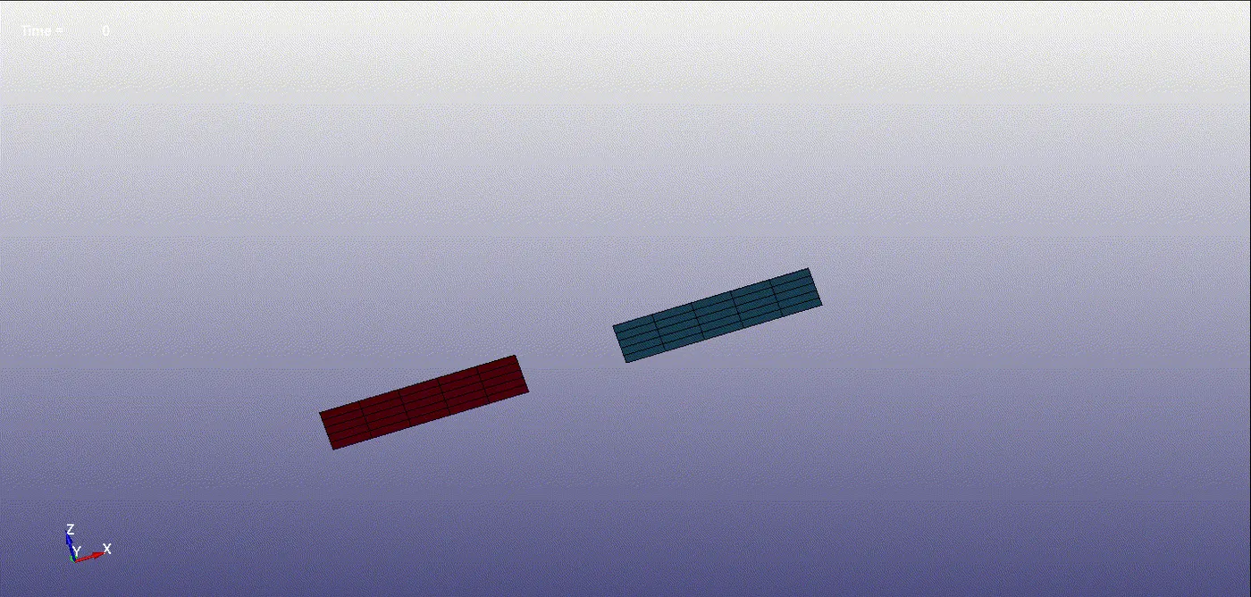
First, 2 shell parts were created using the 4N shell option in the Shape Mesher tab. The two shell parts were separated by appropriate distance, by chosing the appropriate node coordinates.

The shell parts were alloted shell section with 1 mm thickness. The material chosen was MAT_020 Rigid material.

Then, using the Node_Edit option in the Element_tool tab from the right toolbar, 4 nodes were created within the space separating the 2 shell parts. The 4 nodes had 2 pairs of co-incident nodes, created by specifying the same coordinates for each pair.

Then the 2 sets of nodes were created. Each node set had 2 nodes, which were colinear and not coincident. These node sets were added to respective shell parts using the *CONSTRAINED_EXTRA_NODE_SET keyword.

Then, the *CONSTRAINED_JOINT_REVOLUTE keyword was used to create the revolute joint. In this card, the 4 nodes created above were specified, wherein N1 (node 1) and N3 belonged to one shell part, while N2 and N4 belonged to the other.

To prove the working of the joint, it was necessary to provide necessary boundary conditions, control conditions and database requests, which were provided as below:

The *CONTROL_HOURGLASS was provided to avoid hourglassing. The termination time was provided as 1 ms.

For the boundary conditions, the nodes on all 4 sides of a shell part were selected using "By path" option in node selection. These nodes were provided the Single point constraint (SPC) with all 6 DOFs constrained.

As the shell parts were lying in XY plane, on the other shell part, all the nodes on one side of the part were given displacement in z-direction by defining the displacement curve.

The model was run. However, there was error termination. The error read "redundant boundary conditions on nodes". To avoid this error, the boundary conditions were modified. For the SPC, the nodes adjacent to the joint were excluded and only the remaining nodes were given the spc. Also only one node on the other shell part was given translational motion in z-direction, instead of all the nodes on the side of the part.

The model was run. It ran smoothly, but the d3 plot showed only 2 timesteps. Hence to avoid this, the *CONTROL_TIMESTEP keyword was used, in which the timestep curve was provided. The curve was defined using *DEFINE_CURVE, in which the timestep size was kept constant at 1 e-04 ms.

Then the model ran smoothly and there was normal termination. The GIF of the working of the joint is provided below:

Case 2: Deformable bodies

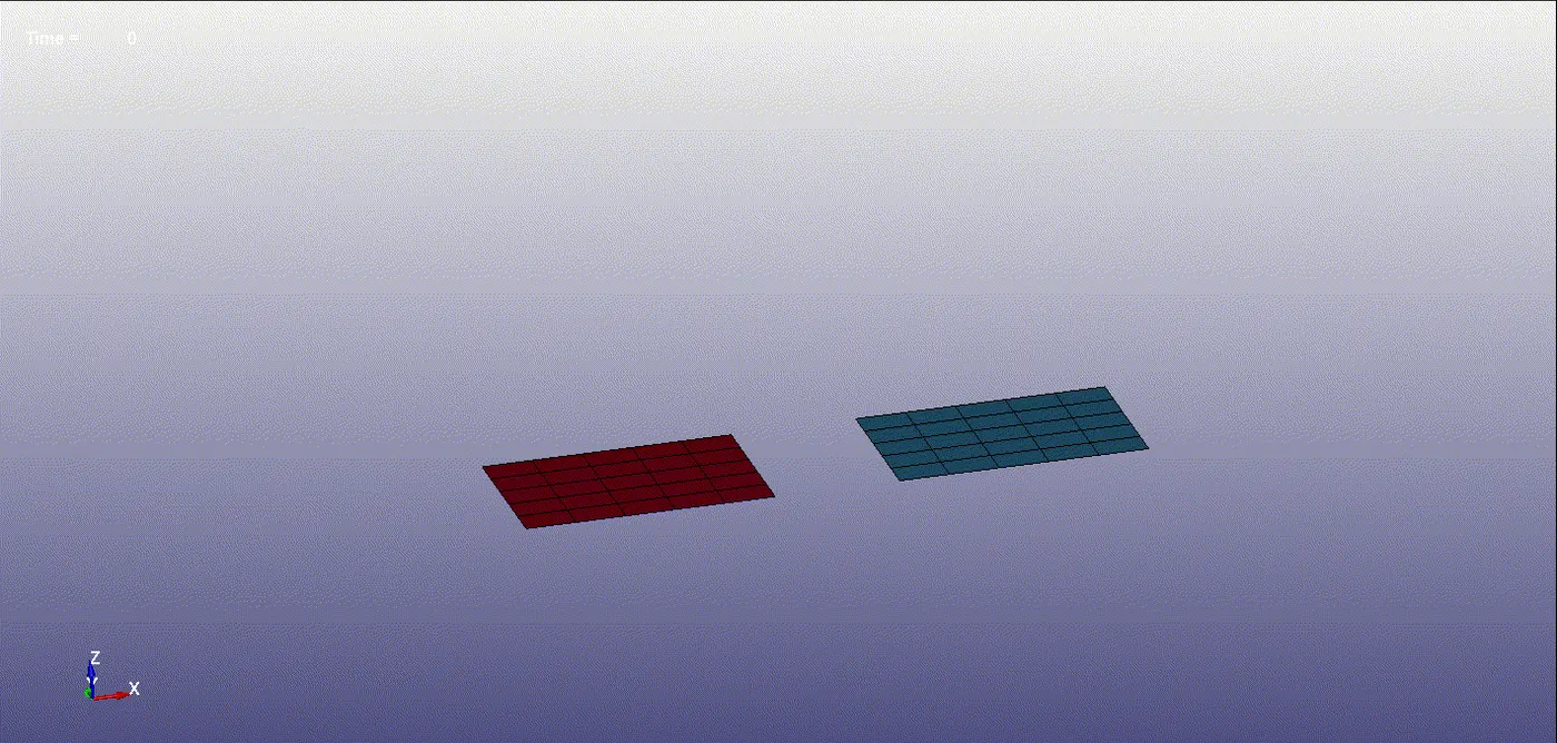
First, 2 shell parts were created using the 4N shell option in the Shape Mesher tab. The two shell parts were separated by appropriate distance, by chosing the appropriate node coordinates.

The shell parts were alloted shell section with 1 mm thickness. The material chosen was MAT_001 Elastic material. The properties of steel were used.

Then, using the Node_Edit option in the Element_tool tab from the right toolbar, 4 nodes were created within the space separating the 2 shell parts. The nodes were not co-incident.

Then the Create_Entity tab was opened to create the CONSTRAINED_NODAL_RIGID_BODY (CNRB). In the CNRB tab, "CrePNode" option was unchecked to avoid creation of CNRB at the center of mass of the selected nodes.

Then one of the created nodes was first selected and then the corresponding nodes for the CNRB were selected. This created the CNRB at the newly created node. The same procedure was repeated for remaining 3 nodes.

Then, in Element_Tools tab, Transform option was used to translate the CNRB's so that 2 CNRBs, one each from the 2 shell parts become co-incident.

Then, the *CONSTRAINED_JOINT_REVOLUTE keyword was used to create the revolute joint. In this card, the node IDs of the 4 CNRBs created above were specified, wherein N1 (node 1) and N3 belonged to one shell part, while N2 and N4 belonged to the other.

To prove the working of the joint, it was necessary to provide necessary boundary conditions, control conditions and database requests, which were provided as below:

The *CONTROL_HOURGLASS was provided to avoid hourglassing. The termination time was provided as 1 ms. The *CONTROL_TIMESTEP keyword was used, in which the timestep curve was provided. The curve was defined using *DEFINE_CURVE, in which the timestep size was kept constant at 1 e-04 ms.

For the SPC, the nodes adjacent to the joint were excluded and only the remaining nodes were given the spc. The nodes were selected using "By path" option in node selection. These nodes were provided the Single point constraint (SPC) with all 6 DOFs constrained.

As the shell parts were lying in XY plane, on the other shell part, one of the nodes on one side of the part were given displacement in z-direction by defining the displacement curve.

Then the model ran smoothly and there was normal termination. The GIF of the working of the joint is provided below:

2. Cylindrical joint

Case 1: Rigid bodies

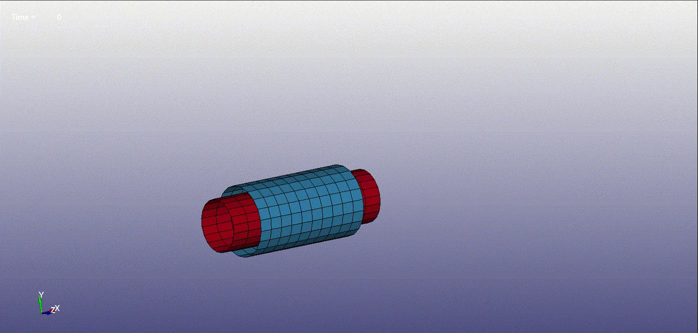
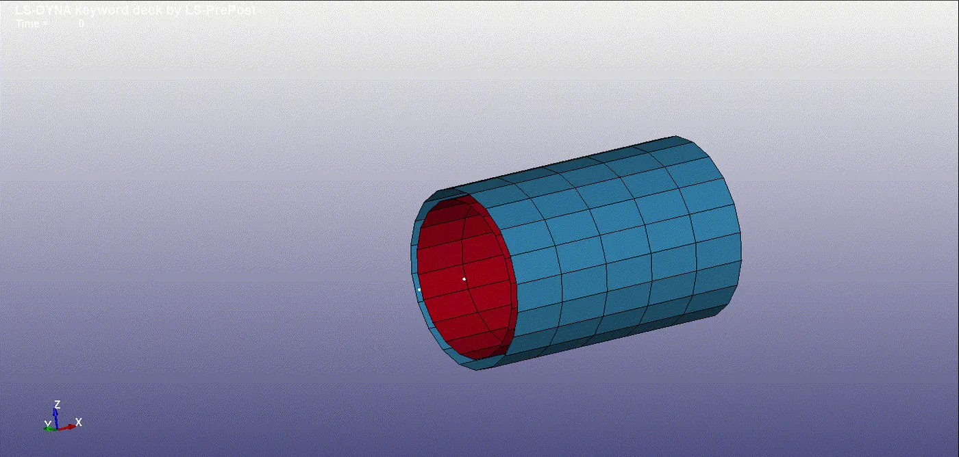
First, 2 shell cylinders were created using the cylinder shell option in the Shape Mesher tab. The two cylinders were co-axial. The outer cylinder has the radius of 17 mm and the inner one has the radius of 15 mm.

The cylinders were alloted shell section with 1 mm thickness. The material chosen was MAT_020 Rigid material.

Then, using the Node_Edit option in the Element_tool tab from the right toolbar, 4 nodes were created within the space inside the inner cylinder. The 4 nodes had 2 pairs of co-incident nodes, created by specifying the same coordinates for each pair.

Then the 2 sets of nodes were created. Each node set had 2 nodes, which were colinear and not coincident. These node sets were added to respective cylinder parts using the *CONSTRAINED_EXTRA_NODE_SET keyword.

Then, the *CONSTRAINED_JOINT_REVOLUTE keyword was used to create the revolute joint. In this card, the 4 nodes created above were specified, wherein N1 (node 1) and N3 belonged to one part, while N2 and N4 belonged to the other.

To prove the working of the joint, it was necessary to provide necessary boundary conditions, control conditions and database requests, which were provided as below:

The *CONTROL_HOURGLASS was provided to avoid hourglassing. The termination time was provided as 10 ms.

For the boundary conditions, the nodes on the circular edge of the outer cylinder were selected using "By path" option in node selection. These nodes were provided the Single point constraint (SPC) with all 6 DOFs constrained.

All the nodes on the circular edge of the other part were given rotation about x-axis by defining the rotation curve. The rotation curve was defined using *DEFINE_CURVE keyword. At 0 ms the rotation was 0 degrees. At 10 ms it was 25 degrees and at 10.1 ms also it was 25 degrees.

The model ran smoothly and there was normal termination. The GIF of the working of the joint is provided below:

Case 2: Deformable bodies

First, 2 shell cylinders were created using the cylinder shell option in the Shape Mesher tab. The two cylinders were co-axial. The outer cylinder has the radius of 17 mm and the inner one has the radius of 15 mm.

The cylinders were alloted shell section with 1 mm thickness. The material chosen was MAT_001 Elastic material.

Then, using the Node_Edit option in the Element_tool tab from the right toolbar, 4 nodes were created on the axis of the 2 cylinders. The nodes were not co-incident.

Then the Create_Entity tab was opened to create the CONSTRAINED_NODAL_RIGID_BODY (CNRB). In the CNRB tab, "CrePNode" option was unchecked to avoid creation of CNRB at the center of mass of the selected nodes.

Then one of the created nodes was first selected and then the corresponding nodes for the CNRB were selected. This created the CNRB at the newly created node. The same procedure was repeated for remaining 3 nodes.

Then, in Element_Tools tab, Transform option was used to translate the CNRB's so that 2 CNRBs, one each from the 2 cylinders become co-incident.

Then, the *CONSTRAINED_JOINT_REVOLUTE keyword was used to create the revolute joint. In this card, the node IDs of the 4 CNRBs created above were specified, wherein N1 (node 1) and N3 belonged to one cylinder, while N2 and N4 belonged to the other.

To prove the working of the joint, it was necessary to provide necessary boundary conditions, control conditions and database requests, which were provided as below:

The *CONTROL_HOURGLASS was provided to avoid hourglassing. The termination time was provided as 10 ms.

For the boundary conditions, the nodes on the circular edge of the innner cylinder were selected using "By path" option in node selection. These nodes were provided the Single point constraint (SPC) with all 6 DOFs constrained.

All the nodes on the circular edge of the other part were given rotation about x-axis by defining the rotation curve. The rotation curve was defined using *DEFINE_CURVE keyword. At 0 ms the rotation was 0 degrees. At 10 ms it was 25 degrees and at 10.1 ms also it was 25 degrees.

The model ran smoothly and there was normal termination. The GIF of the working of the joint is provided below:

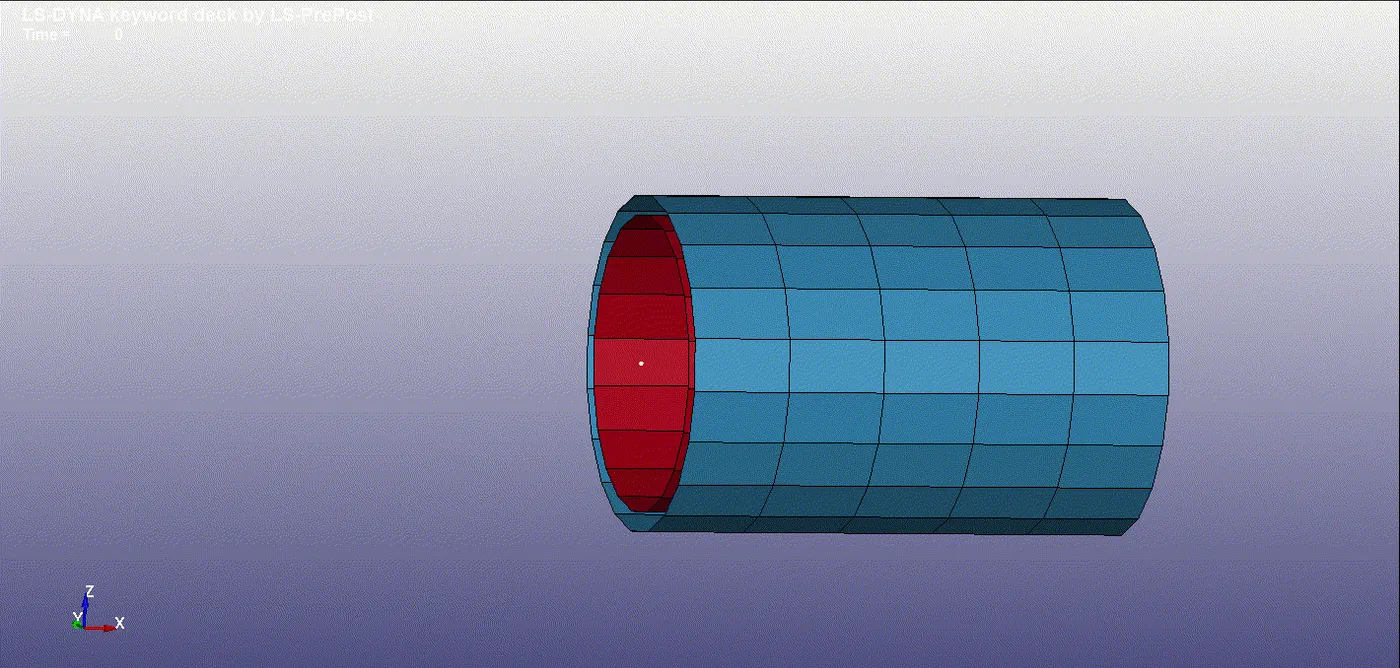
For both the cases above, the translational motion was also checked. The GIF for the same is attached below:

3. Spherical joint

Case 1: Rigid bodies

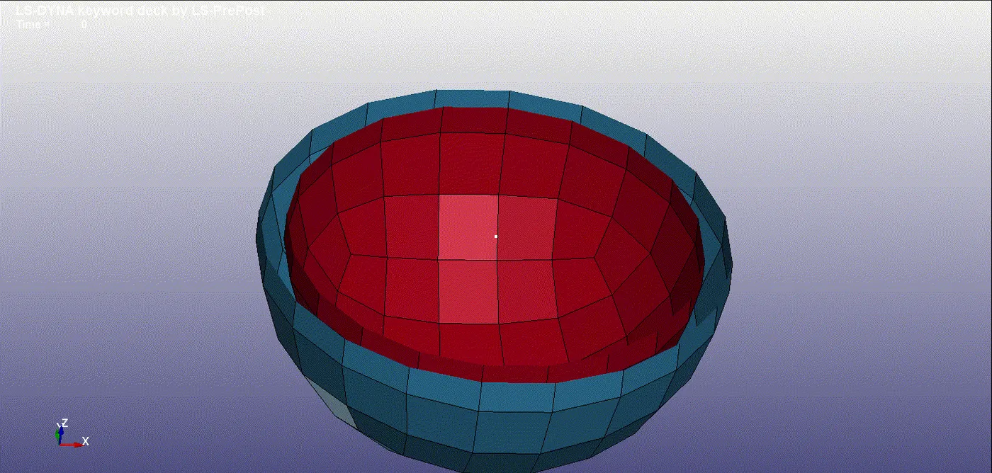
First, 2 shell spheres were created using the sphere shell option in the Shape Mesher tab. The origins of the two spheres were coincident. The outer sphere has the radius of 17 mm and the inner one has the radius of 15 mm.

The spheres were allotted shell section with 1 mm thickness. The material chosen was MAT_020 Rigid material.

Then, using the Node_Edit option in the Element_tool tab from the right toolbar, 2 nodes were created within the inner sphere at the origin. The nodes were co-incident, created by specifying the same coordinates for each pair.

These nodes were added to respective spheres using the *CONSTRAINED_EXTRA_NODE_SET keyword.

Then, the *CONSTRAINED_JOINT_SPHERICAL keyword was used to create the spherical joint. In this card, the 2 nodes created above were specified, wherein N1 (node 1) belonged to one part, while N2 belonged to the other.

To prove the working of the joint, it was necessary to provide necessary boundary conditions, control conditions and database requests, which were provided as below:

The *CONTROL_HOURGLASS was provided to avoid hourglassing. The termination time was provided as 1 ms.

For the boundary conditions, the nodes on the inner sphere were selected using "By part" option in node selection. These nodes were provided the Single point constraint (SPC) with all 6 DOFs constrained.

All the nodes on the other part were given rotation about z-axis by defining the rotation curve. The rotation curve was defined using *DEFINE_CURVE keyword. At 0 ms the rotation was 0 degrees. At 1 ms it was 50 degrees and at 1.1 ms also it was 50 degrees.

The model ran smoothly and there was normal termination. The GIF of the working of the joint is attached.

Case 2: Deformable bodies

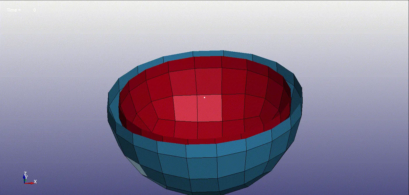
First, 2 shell spheres were created using the sphere shell option in the Shape Mesher tab. The origins of the two spheres were coincident. The outer sphere has the radius of 17 mm and the inner one has the radius of 15 mm.

The spheres were allotted a shell section with 1 mm thickness. The material chosen was MAT_001 Elastic material.

Then, using the Node_Edit option in the Element_tool tab from the right toolbar, 2 nodes were created within the inner sphere at the origin. Initially, the nodes were not coincident.

Then the Create_Entity tab was opened to create the CONSTRAINED_NODAL_RIGID_BODY (CNRB). In the CNRB tab, "CrePNode" option was unchecked to avoid creation of CNRB at the center of mass of the selected nodes.

Then one of the created nodes was first selected and then the nodes on one of the spherical bodies were selected using “By part” option. This created the CNRB at the newly created node. The same procedure was repeated for the remaining node.

Then, in Element_Tools tab, Transform option was used to translate the CNRB's so that 2 CNRBs, become co-incident.

Then, the *CONSTRAINED_JOINT_SPHERICAL keyword was used to create the spherical joint. In this card, the node IDs of the 2 CNRBs created above were specified, wherein N1 (node 1) belonged to one sphere, while N2 belonged to the other.

To prove the working of the joint, it was necessary to provide necessary boundary conditions, control conditions and database requests, which were provided as below:

The *CONTROL_HOURGLASS was provided to avoid hourglassing. The termination time was provided as 1 ms.

For the boundary conditions, the nodes on the inner sphere were selected using "By part" option in node selection. These nodes were provided the Single point constraint (SPC) with all 6 DOFs constrained.

All the nodes on the other part were given rotation about z-axis by defining the rotation curve. The rotation curve was defined using *DEFINE_CURVE keyword. At 0 ms the rotation was 0 degrees. At 1 ms it was 50 degrees and at 1.1 ms also it was 50 degrees.

The model ran smoothly and there was normal termination. The GIF of the working of the joint is provided below:

4. Translational joint

Case 1: Rigid bodies

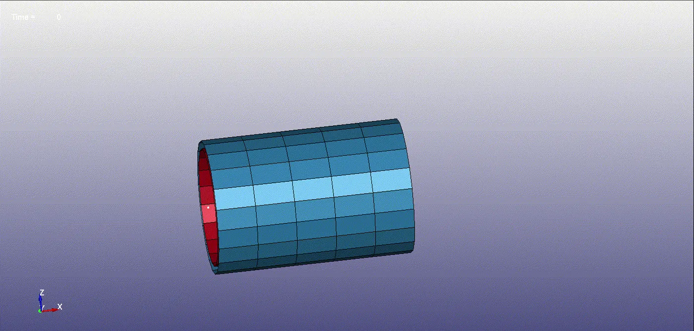
First, 2 shell cylinders were created using the cylinder shell option in the Shape Mesher tab. The two cylinders were co-axial. The outer cylinder has the radius of 17 mm and the inner one has the radius of 15 mm.

The cylinders were alloted shell section with 1 mm thickness. The material chosen was MAT_020 Rigid material.

Then, using the Node_Edit option in the Element_tool tab from the right toolbar, 6 nodes were created within the space inside the inner cylinder. The 6 nodes had 3 pairs of co-incident nodes, created by specifying the same coordinates for each pair. The 4 of the 6 nodes were on the axis of the cylinders, while the 2 were offset from the axis.

Then the 2 sets of nodes were created. Each node set had 3 nodes, which were colinear and not coincident. These node sets were added to respective cylinder parts using the *CONSTRAINED_EXTRA_NODE_SET keyword.

Then, the *CONSTRAINED_JOINT_TRANSLATIONAL keyword was used to create the translational joint. In this card, the 6 nodes created above were specified, wherein N1 (node 1), N3 and N5 belonged to one part, while N2, N4 and N6 belonged to the other.

To prove the working of the joint, it was necessary to provide necessary boundary conditions, control conditions and database requests, which were provided as below:

The *CONTROL_HOURGLASS was provided to avoid hourglassing. The termination time was provided as 1 ms.

For the boundary conditions, the nodes on the circular edge of the inner cylinder were selected using "By path" option in node selection. These nodes were provided the Single point constraint (SPC) with all 6 DOFs constrained.

All the nodes on the circular edge of the other part were given translation along x-axis by defining the displacement curve. The displacement curve was defined using *DEFINE_CURVE keyword. At 0 ms the displacement was 0 mm. At 1 ms it was 50 mm and at 1.1 ms also it was 50 mm.

The model ran smoothly and there was normal termination. The GIF of the working of the joint is provided below:

Case 2: Deformable bodies

First, 2 shell cylinders were created using the cylinder shell option in the Shape Mesher tab. The two cylinders were co-axial. The outer cylinder has the radius of 17 mm and the inner one has the radius of 15 mm.

The cylinders were alloted shell section with 1 mm thickness. The material chosen was MAT_001 Elastic material.

Then, using the Node_Edit option in the Element_tool tab from the right toolbar, 6 nodes were created within the space inside the inner cylinder. The 6 nodes had 3 pairs of co-incident nodes, created by specifying the same coordinates for each pair. The 4 of the 6 nodes were on the axis of the cylinders, while the 2 were offset from the axis.

Then the Create_Entity tab was opened to create the CONSTRAINED_NODAL_RIGID_BODY (CNRB). In the CNRB tab, "CrePNode" option was unchecked to avoid creation of CNRB at the center of mass of the selected nodes.

Then one of the created nodes was first selected and then the nodes on one of the cylindrical bodies were selected using “By path” option. This created the CNRB at the newly created node. The same procedure was repeated for the remaining 5 nodes.

Then, in Element_Tools tab, Transform option was used to translate the CNRB's so that the respective pairs of CNRBs become coincident.

Then, the *CONSTRAINED_JOINT_TRANSLATIONAL keyword was used to create the translational joint. In this card, the 6 nodes created above were specified, wherein N1 (node 1), N3 and N5 belonged to one part, while N2, N4 and N6 belonged to the other.

To prove the working of the joint, it was necessary to provide necessary boundary conditions, control conditions and database requests, which were provided as below:

The *CONTROL_HOURGLASS was provided to avoid hourglassing. The termination time was provided as 1 ms.

For the boundary conditions, the nodes on the circular edge of the inner cylinder were selected using "By path" option in node selection. These nodes were provided the Single point constraint (SPC) with all 6 DOFs constrained.

All the nodes on the circular edge of the other part were given translation along x-axis by defining the displacement curve. The displacement curve was defined using *DEFINE_CURVE keyword. At 0 ms the displacement was 0 mm. At 1 ms it was 50 mm and at 1.1 ms also it was 50 mm.

The model ran smoothly and there was normal termination. The GIF of the working of the joint is provided below:

Conclusion:

The challenge was a useful lesson on how to model different types of joints in LS-Dyna. Also it underscored the importance of referring to the LS-Dyna manual, while using the software. Along with the joints, the challenge provided an opportunity to learn keywords like Constrained_extra_nodes, control_timestep, constrained_nodal_rigid_body etc. It also allowed one to learn about the “Node_edit” option and how to translate nodes using “transform” command. It also provided lessons about using the “Shape mesher” option. All in all, the challenge was a great learning experience.