Week 11: FSAE Car Project

Flow over a FSAE car model

• Aim:

Perform an external flow simulation over a FSAE car model. Initially perform geometry clean-up to remove mani-fold edges and overlapping trias. Assign different components different boundary flagging and create a wind tunnel around the FSAE car model to perform external aerodynmics simulations.

• Theory:

1. FSAE car model:

Formula SAE is a student design competition organized by SAE International (previously known as the Society of Automotive Engineers, SAE). The competition was started in 1980 by the SAE student branch at the University of Texas at Austin after a prior asphalt racing competition proved to be unsustainable.

The concept behind Formula SAE is that a fictional manufacturing company has contracted a student design team to develop a small Formula-style race car. The prototype race car is to be evaluated for its potential as a production item. The target marketing group for the race car is the non-professional weekend autocross racer. Each student team designs, builds and tests a prototype based on a series of rules, whose purpose is both ensuring on-track safety (the cars are driven by the students themselves) and promoting clever problem solving.

2. Downforce:

Downforce is a downwards lift force created by the aerodynamic features of a vehicle. If the vehicle is a car, the purpose of downforce is to allow the car to travel faster by increasing the vertical force on the tires, thus creating more grip. If the vehicle is a fixed-wing aircraft, the purpose of the downforce on the horizontal stabilizer is to maintain longitudinal stability and allow the pilot to control the aircraft in pitch.

• Procedure:

1. Upload the geometry onto converge studio v3.0, remove the overlapping edges and non-manifold edges uising the geometry editing tools and assign the entire car to a single boundary.

2. Assinging boundary flags for different components of the car can be done by using boundary fencing, where we create a fence around different boundaries to flagged and select that boundary using boundary fencing selection.

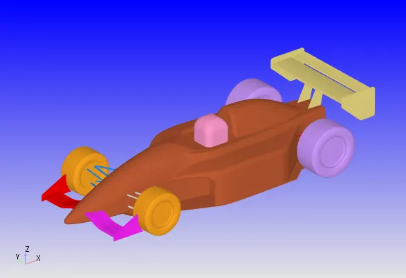
3. After assigning the boundary we have to delete the flat surface the tyre so that wind tunnel and the tyre surface do not coincide to create a meshing error.

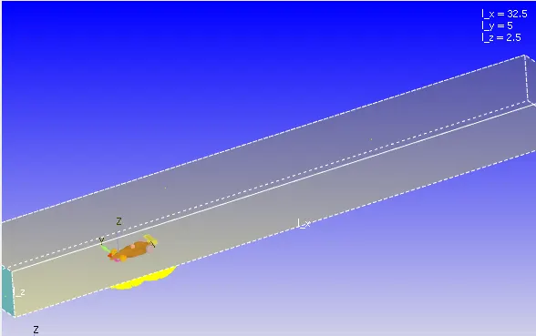
4. After locating the lowest vertical point of the car model, we need to create a wind tunnel with reference to the standard measurements and create triangles and edges to complete the wind tunnel.

-Case setup:

- Initially running the simulation on steady state, the results were not satisfying. It caused errors at the finer regions of the mesh and closer values at the coarse mesh which contradicts the theory, since steady state is time independent and tries to solve the domain fast as possible without considering the flow physics more precisely, therefore transient simulation is considered since we are interested in finding the flow physics and flow seperation more accurately along the path of simulation for analysis.

- Transient case setup:

1. Application type: time based

2. Materials:

a. Gas simulation: air

b. Global transport properties: Deafult

c. Species: O2 and N2

3. Simulation parameters:

a. Run parameters:

Transient solver, full hydrodynamic, compressible

b. Simulation time parameters:

- End time- 2 sec

Calculating end time:

End time is calculated by analysing the flow time from the inlet to outlet and the inlet velocity at which the flow generates, by knowing these 2 parameters, we can calculate the end time.

Since, length of the pipe is approx 32.5m and velocity at inlet = 20.83 m/s(straights), 12.5m/s(lot of turns)

Therefore, end time = distance of pipe/ inlet velocity

Which implies,

for straigths, 32.5/20.83= 1.5 sec

for lot of turns, 32.5/12.5= 2.6sec

It takes 1.5 and 2.6 secs for the flow to complete 1 cycle

- Time step- 1e-6

- min time step- 1e-6

- max time step- 1

- Convection CFL number- 0.5

c. Solver Parameters-

- Solver type- density based solver

4. Boundary Conditions-

a. Inlet- Inflow

- Total pressure- NE

- Inlet velocity- 20.83, 12.5m/s

- Initial temp- 300K

- Species boundary condition- add air

b. Outlet- Outflow

- Pressure- NE

- Backflow - temp= 300k

- add air

c. No-Slip bottom surface - Wall, no-slip BC

no slip condition- The contact region between wall surface and fluid region tends to create high friction and create a 0 velocity of fluid flow, and due to viscosity of fluid, the fluid layers tend to undergo shear stress and have high pressure and overlap on eachother which eventually forms a fully developed region where velocity is max and constant and having low pressure.

d. Slip bottom surface- Wall

- Slip BC

e. Wall Symmetry(sides and top)- Symmetry BC

- Symmetry

f. FSAE car (all the components) - Wall

- Law of the wall

- Omega wall conditions: Wall model

5. Initial Conditions and Events:-

- Regions and Initialization:

x-velocity: 20.83, 12.5m/s

Pressure- 1.5e5 Pa

Temperature: 300K

Add- air

6. Physical Models:-

- RANS k-w SST

7. Grid Control:-

a. Base Grid:

dx = 2e-4m, dy = 2e-4m, dz = 2e-4m

b. Embedding:

- Box embedding

- Boundary embedding: FASE Body, permanent mode embedding.

Scale- 3

Number of layers- 6

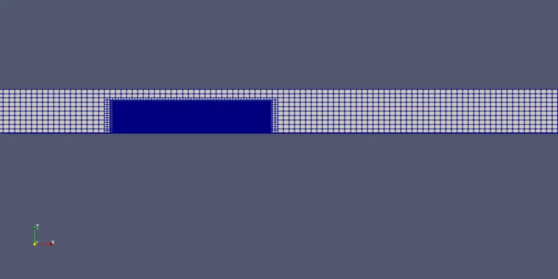
Embedding is the means by which we can refine the mesh to a value that is lower than the prevalent base size. This is especially useful if we are looking to refine near wall to capture the boundary layer or the wake of a body more accurately.

8. Post-Processing:-

- Post Variable Selection:

Select the parameters needed to be post processed.

- Output files:

- Enable Boundaries only under wall output in output generation,this helps us to get averaged values of certain physical quantities.

We need to set a time interval for the files to be saved during each set of iterations. It is best suited to have a min of 100 saved files for every simulation. Therefore we need to calculate the time interval for writing the output files based on our end time given in run parameters.

Restart files help in restoring the files if there is a sudden power cut/ crash which is not helpful or might end up loosing the entire data, therefore the restart files helps in resuming the simulation form the point we lost contact. Restart files time interval can be same as the writing files interval which is safe and healthy.

In this case- since the end time is 1.5 and 2.6, we can have a time interval of 0.015 and 0.026 and the total files created will be 100.

• Results:

1. Straight path:

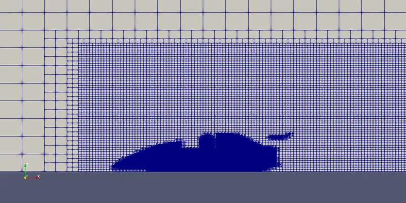
a. Mesh:

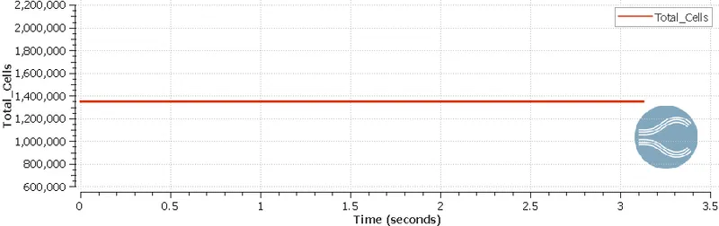
- Total cell count:

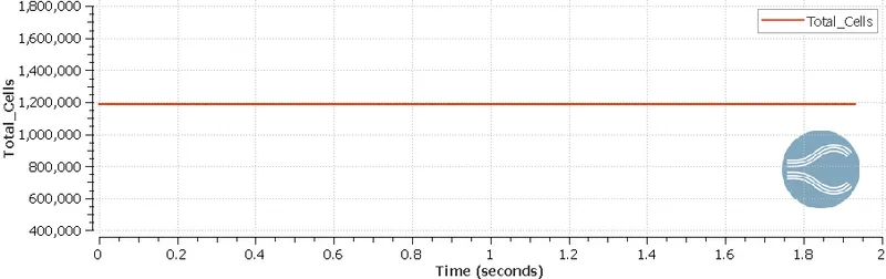
The entire geometry was discretized into finite number of cells or elements. Above plot shows the number of cells or elements created. The total cell-count is constant throughout the simulation.

In first case, since we are doing an external aerodynamic simulation it is important for us to capture the data accurately and in time to time. So the cell count should be higher in order to these functions.

Around 1.2 to 1.35 million cells were created in the simulation.

b. Velocity plots and contours:

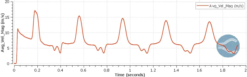
- Velocity magnitude variation at body:

- Velocity contours:

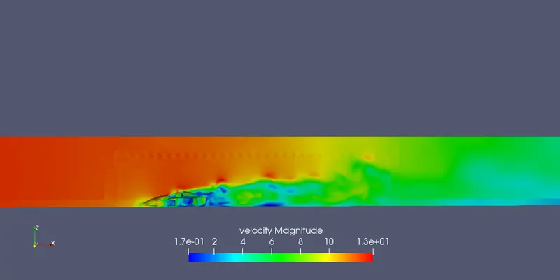
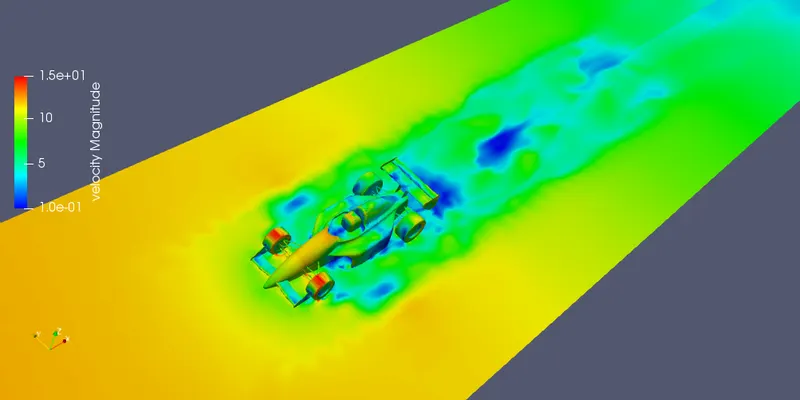
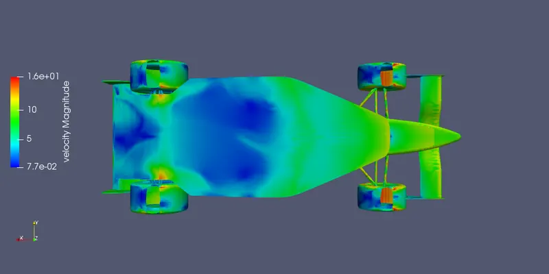
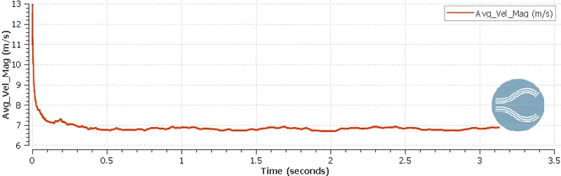
When a flow over 20.83 m/s encounters a car or in other words when a car moves at a speed of 20.83 m/s its's velocity over the wheels increases. The velocity at the back end of the car is low and also at the contacts where the wheels are touching the ground, velocity is low (about 14 m/s).

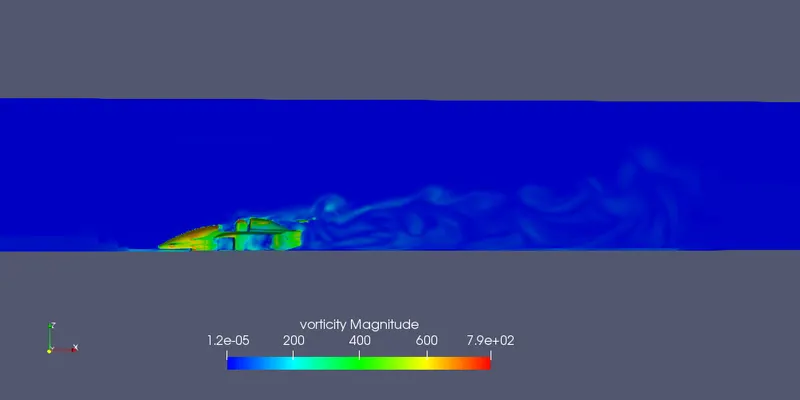
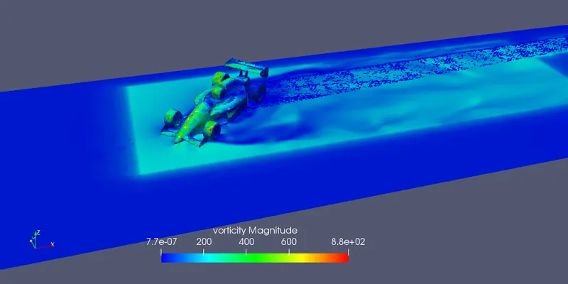
- Vorticity:

Vorticity is the rate at which the fluid spins on the surface of the body. In fluid mechanics, vorticity is a psuedo vector field that describes the local spinning motion of a continuum near some point (the tendency of something to rotate, as would be seen by an observer located at that point and traveling along with the flow.

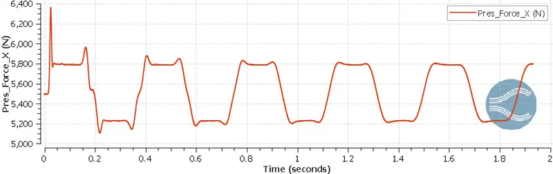
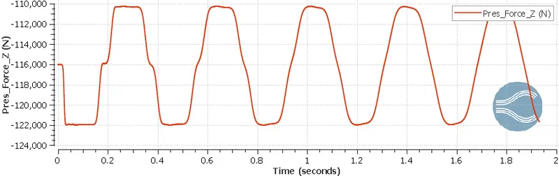
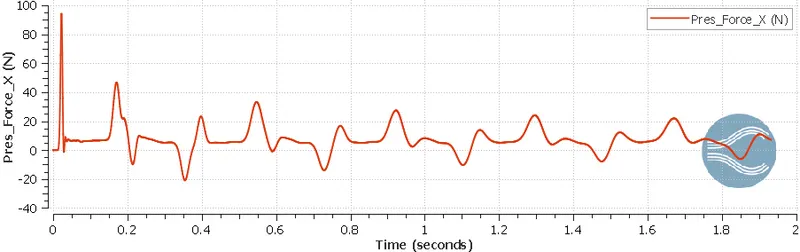
- Drag force and Downforce at different parts of the car model:

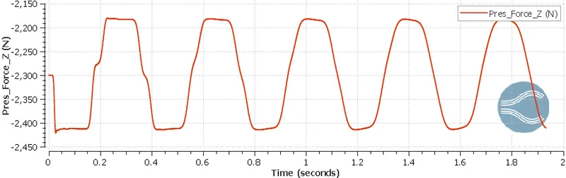
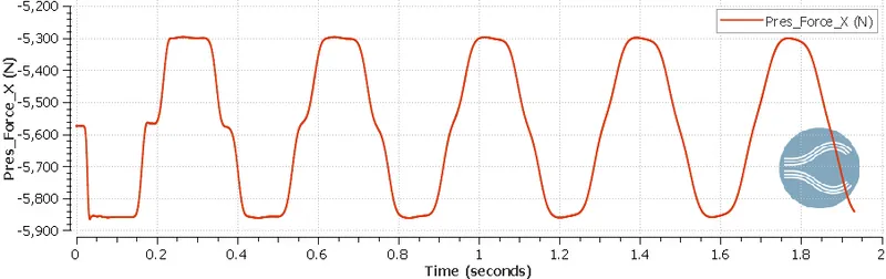
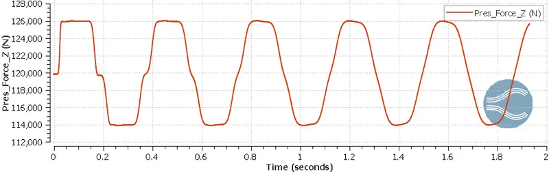
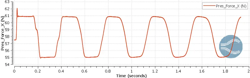
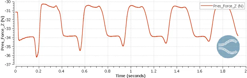
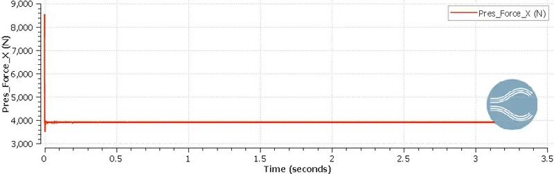
Pressure force_X = Drag force

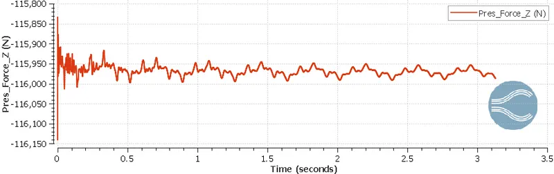
Pressure force_Z = Downforce

a. Body:

b. Front wheels:

c. Rear wheels:

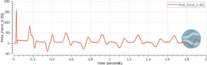
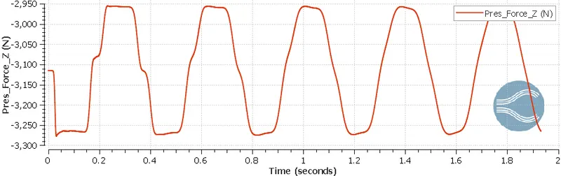
d. Rear wing:

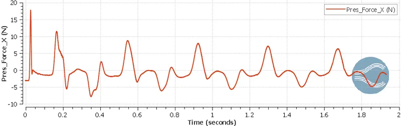
e. Underbody:

f. Front wings:

- Streamline:

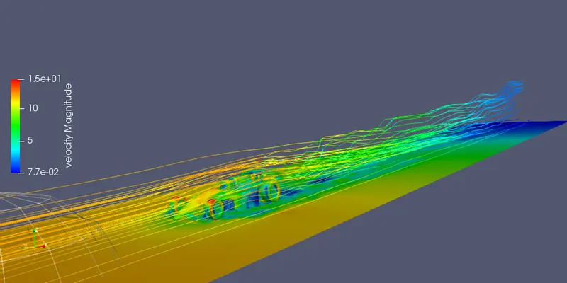
2. Lot of turns path:

a. Mesh:

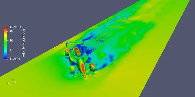
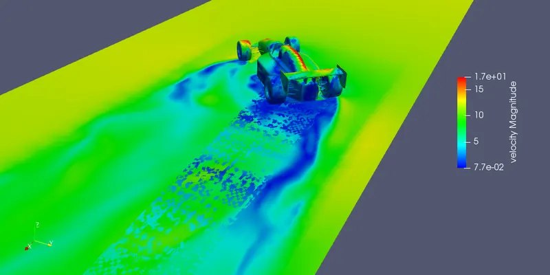
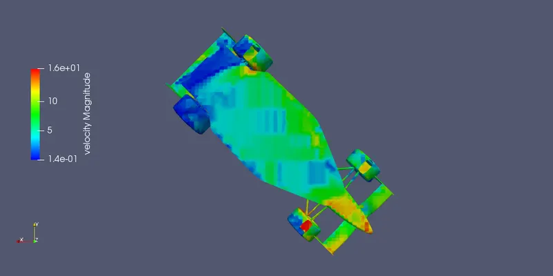
- Velocity:

- Velocity magnitude at front wheels:

- Contours:

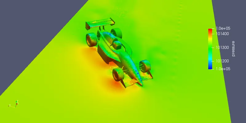
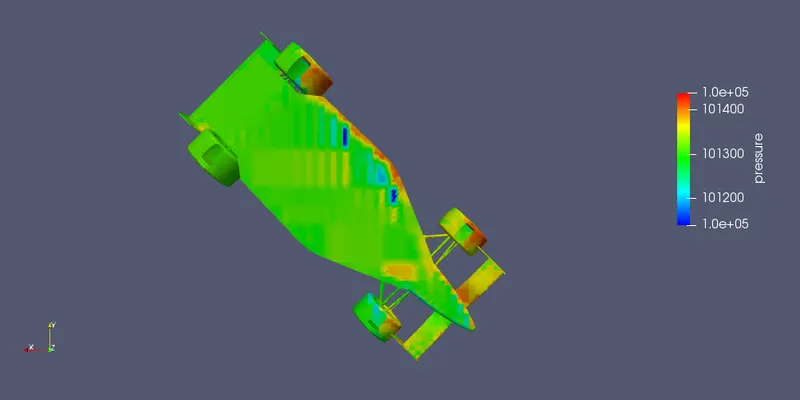
- Pressure:

- Vorticity:

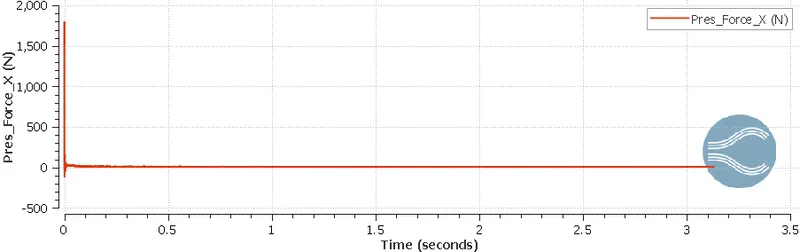
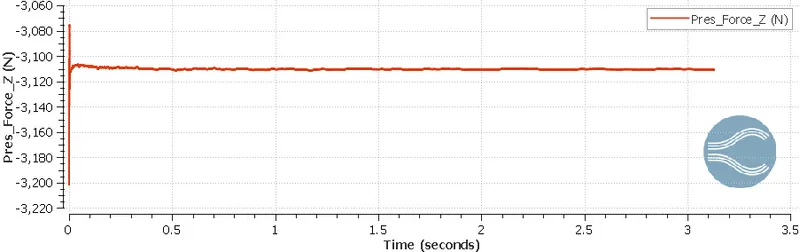
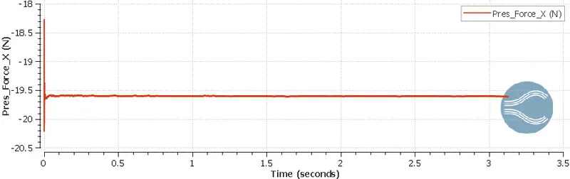
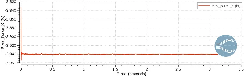
- Drag force and Downforce at different parts of the car model:

Pressure force_X = Drag force

Pressure force_Z = Downforce

a. Body:

b. Rear Wing:

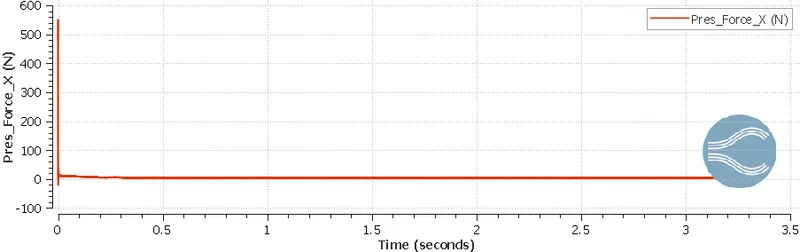
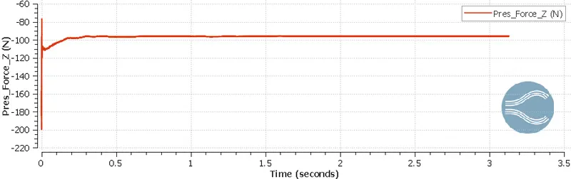
c. Front wheels:

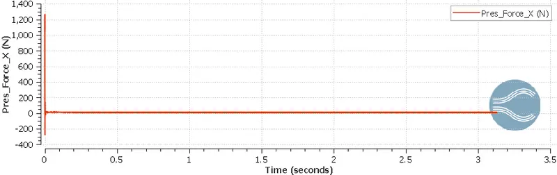
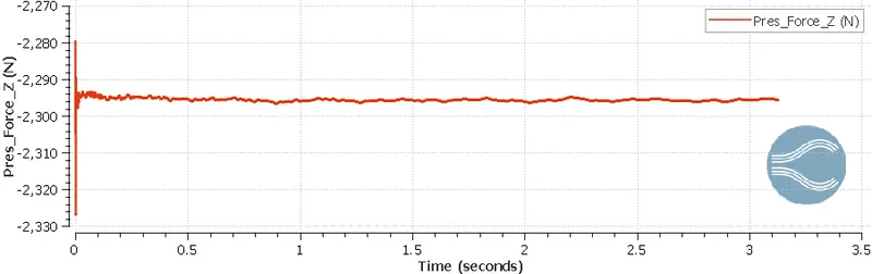
d. Rear wheels:

e. Front wings:

Drag force front wheel left:

Drag force front wheel right:

Down force front wing left:

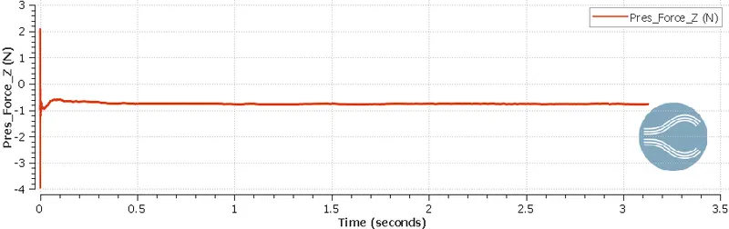
Down force front wing right:

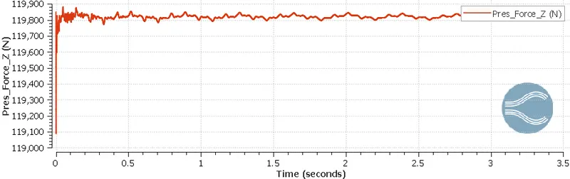
- Streamline:

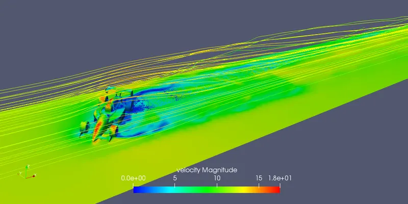
Atthe rea end of the FSAE car the flow is recirculating over the rear wheels and the rear wing and also there is a region just below the rear wing where the flow is getting recirculated and is pointing

towards the rear wing, if this happens some amount of lift will be generated which destroys the tendency of the car to bite or stay on the ground.

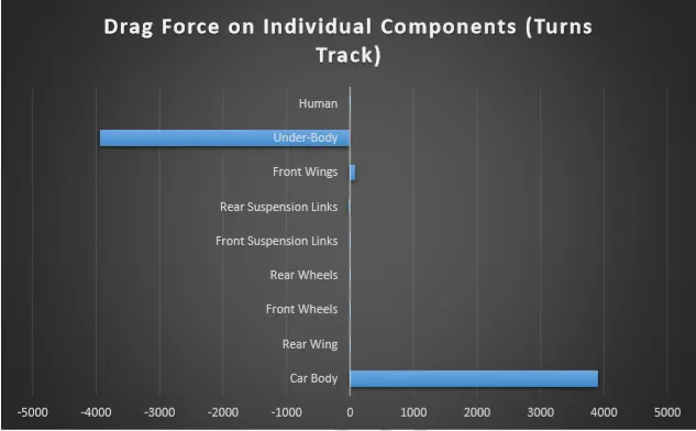
- Drag force chart:

- Down Force chart:

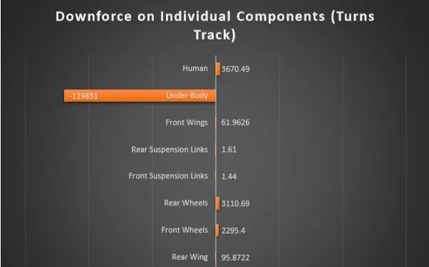
- DOWN FORCE-DRAG FORCE (RATIO)

Component name	Down force (N)	Drag force (N)	Down force : Drag force (RATIO)
Car body	115982	3914.6	29.62
Rear wing	95.362	3.6	25.20
Front wheels	2265.4	9.1	230.50
Rear wheels	3100.59	7.68	389.22
Front suspension links	1.34	4.56	0.311
Rear suspension links	1.85	-30.50	0.322
Front wings	61.96	83.5	0.752
Under-body	-119831	-3948.25	30.504
Human	3680.49	1.6	2353.81

• Conclusion

After analyzing the data and the result, it was observed that wheels or tires generated a portion of overall drag. To reduce drag on tire, wheels can be covered to make it more aerodynamic. Due to regulation, full covering might not be allowed, but if partial bodywork is permitted, placing converging fairing behind the wheels provides maximum benefit.

According to the result observed in front wing, it did not generate much downforce than needed, thus, the front wing should be designed aerodynamically to increase the overall downforce on the car.

The car body was rotated at an angle of 49.5 degree which is a side slip angle and the tire experiences more load because of turning and high-velocity region in the nose and the air ducts then the low-pressure region in the flow separation region streamline visualization will create drag into rn both combine to produce lift. ( Lot of turns)

The flow over wheels where the top surface of the wheel experiences the higher velocity because the flow over there creates the more the flow front wings where high pressure on top and low pressure on the bottom. The two endplates are fixed to prevent the formation vortices here the vortices are seen at the end so additional drag increases. To reduce the drag is to reduce the airfoil thickness and adding flaps like in an airplanes.

The flow over the rear wing as seen that it creates lift force over the corners by seeing the velocity profiles. This because of the generation vortices and the airfoil in the car wing usually have low aspect ratio and in turn, it creates the drag behind the body and also reduces the angle of attack of free stream air. To improve the lift is to increase airfoil thickness and also increase the height of endplate. The Y plus is uniform throughout the body. The forces on the suspension links are very low and there is a need in change of suspension links.