Week-11 Challenge: Braking
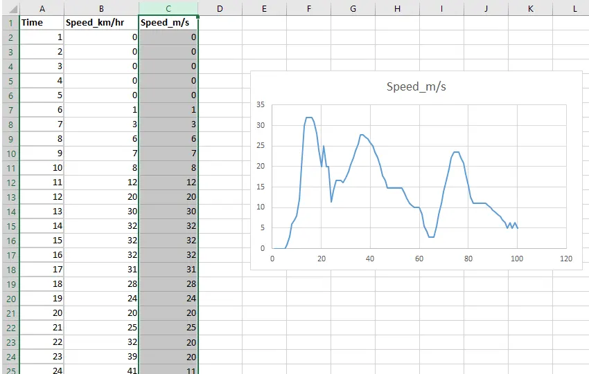
Ans 1: The random driving cycle is created in excel for 100s and defined as follows for the Brake Energy Calculation:
The Brake energy is calculated by the change in Kinetic energy of vehicle at every instant of braking applies as by the general formula
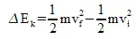
Where m is the mass of the vehicle, lets say 1000kg and Vf and Vi are the next velocity and the last velocity of vehicle during each braking instant.
The Matlab command window is given below to show the import of Driving cycle excel file
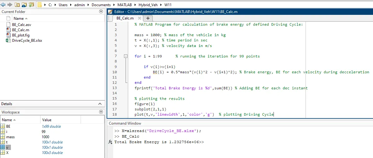
The MATLAB program is written as follows to calculate BE for each instant of decceleration:
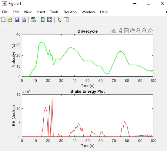
Results: From the below plots, we can verify that the Brake energy is only required during decceleration of the vehicle.
>> X=xlsread('DriveCycle_BE.xlsx');
>> BE_Calc
Total Brake Energy is 1.232756e+06>>
The total Brake Energy is calculated as appx. 1.23MJ.
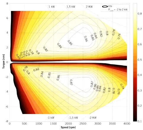
Ans 2: Electric Motor can't develop braking torque at high speed similar to staring. As we can see from the typical speed torque characteristics for both traction and braking below, if, for instance, the braking initiated at high speed of 2000rpm, the torque developed by the motor during traction is around 5Nm @1kW power which is not maximum in this region as compared to the torque developed in braking region. This is due to the reason once the electric supply is cut-off from the motor, it starts acting as a generator and due to the flux weakening effect of the electric generator, the generator produces low torque as expected.
Coordination of Electric and Mechanical Brake :
In an electric Motor, the Total Brake application is distributed in two aspects; first is Electrical Brake which is also called Regenerative Brake, and the second is Mechanical Brake or Classical Brake working on hydraulic cylindrical system.
The strategy of the above two brakes distribution is based on several factors.
For example, if the Regenerative braking power requirement is more than the charging limit of the battery or more than the regenerative capacity of the machine, Mechanical brakes are equivalently applied as well.
In a practical case, the combination of these two is applied. There are two main Brake Control Strategies. Based on the comfort of the driver and energy efficiency, these are applied.
i) Series: Here, Mechanical brake and Regenerative electric brake are applied one after another.
ii)Parallel: Here, both brakes are applied simultaneously.
The Control criteria is adopted such that at low speed use regenerative braking higher and at high speed or during the initial braking period we actually combine the both as shown in the figure below.
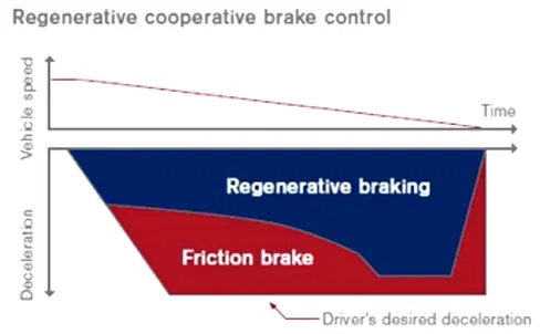
Beacuse for the same reason at high speed, the reverese brake power for charging may exceed the battery charging capacity and may also damage the inverter power electronics circuit.
ANs 3: To find the efficiency of motor, we first need to find the types of losses possible in machine whether BLDC or Induction motor. These are of following four types:
i) Copper loss: Pc= Kc. T^2
ii) Iron Loss: Pi=Ki. w
iii) Windage Loss: Pw=Kw. w^3
iv) Constant Loss: Some fixed loss, K
The total loss is given as
Total Losses = kc⋅T2+ki⋅ω+kw⋅ω3+C">kc⋅T2+ki⋅ω+kw⋅ω3+ K
MATLAB program for calculating the losses and plotting contour of efficiency of the EV motor: