Week-11 Challenge: Braking

(1). For a defined driving cycle, calculate the energy required for braking.

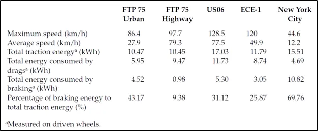
The braking performance is one of the most important concerns in vehicle safety. In urban area driving, a significant amount of energy is consumed in braking. Electrification of vehicles makes it feasible to recover some of the energy lost in braking. A hybrid braking system was developed to ensure the efficient braking of the vehicle and recovering the braking energy. The design and control objectives of such a hybrid braking system are to ensure sufficient braking force to quickly reduce the vehicle speed, properly distributing the brake force to the front and rear axle, and also recover as much braking energy as possible. So understanding of braking energy of a driving cycle is important. Now, it is also important to mention that braking energy also depends upon the type of driving cycle i.e. the higher number of time the vehicle will have rapid speed changes and will come to rest then the braking energy will automatically rise for that particular drive cycle than other driving cycle where the rapid speed changes don't occur.

In electric vehicle is require by vehicle for acceleration as well as deacceleration of vehicle also. As we require to stop vehicle in stipulated time, we cannot allow vehicle to stop as per its inertia value, for stopping vehicle we require to apply brake. Braking of vehicle require to deaccelerate vehicle to lower speed within a given time.

Braking Energy = (1/2)*m*v^2

Where, Braking Energy is the kinetic energy in unit of Joule.

m= Total Mass of the Vehicle (Vehicle Mass + Pay Load) in unit of Kg.

v= (Initial Velocity-final Velocity) in unit m/s.

For Example if Initial speed of a vehicle is 20m/s and final speed is 10m/s. The mass of the vehicle is 1000kg. Then the required kinetic energy for Braking is (1/2)*1000*(20-10)^2 = 50000 J =50KJ

Suppose we have UDDS cycle: -

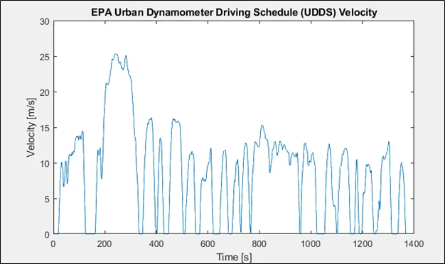
We can observe in this test cycle vehicle needs to stop in given time at some instance also for this we will apply brakes. We will calculate the power require for braking operation.

Please refer the attached sheet for complete calculation of Deacceleration energy require in UDDS cycle.

• To reduce speed from 80 to 40 Kmph in 20 sec = 292 KJ
• To reduce speed from 80 to 0 Kmph in 10 sec = 560 Kj

(2) Why electric motor can’t develop braking torque at high speed similar to starting? How electric and mechanical brakes are coordinated?

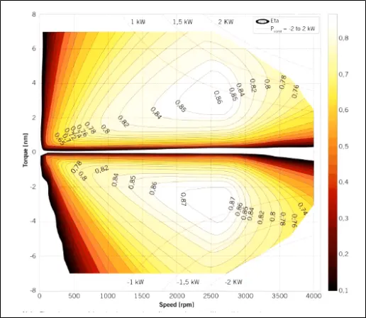
This is torque-speed contour plot of motor.

We can see that, at the time of accelerating vehicle at starting the maximum torque available motor is operating at constant torque region, in that motor will have maximum torque available, but as motor starts deaccelerating motor characteristics are shifted towards braking region, in this we don’t have max torque available for braking as motor is already running at higher speed.

Due to this operation, electric motor can’t develop braking torque at high speed similar to starting

(i) Mechanical Braking:

Mechanical brakes all act by generating frictional forces as two surfaces rub against each other. The stopping power or capacity of a brake depends largely on the surface area of frictional surfaces as well as on the actuation force applied. Mechanical brakes are assemblies consisting of mechanical elements for the slowing or stopping of shafts in equipment drives. They use levers or linkages to transmit force from one point to another. Braking slows or stops the movement of the coupled shafts. There are several types of mechanical brakes.

(ii) Electrical Braking:

Electric brakes are devices that use an electrical current or magnetic actuating force to slow or stop the motion of a rotating component. They are used in industrial and vehicular braking applications that require fast response times and precise tension control. The magnet in the backing plate has 2 conductor wires which tap directly into the wiring. When electricity is on, it magnetizes the brake magnet. The magnet is attracted to the drum face. When it contacts this area, the friction causes it to rotate, which moves the actuating arm, and pushes the shoes out against the drum. Those shoe have a special brake pad material on them that resists the heat caused by that friction. When the shoes press against the inside of the drum, they prevent the hub, and consequently the wheel that's touching the ground.

A very beautiful electric braking scheme called Regenerative Braking is now being employed for electric braking. Here during the braking action, the motor is operated as generator. As we know that during generating action, a counter torque is produced. So this counter torque opposes the motion of motor and motor comes to halt. Moreover, the brake energy is converted to electrical energy which can be fed back to the source using power converters.

Electrical and mechanical braking systems can are coordinated by using Brake strategy subsystem

• Serial Braking Strategy
• Parallel Braking Strategy

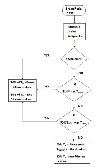
serial braking strategy

• Once the brake pedal is pressed and depending on the level of depression, a brake torque is sent.
• Now this brake torque passes into the brake control strategy block. Here, firstly it is checked if battery state-of-charge is below 80% which is set as the maximum permissible level of charge. If that condition is satisfied, then the battery is recharged.
• The brake torque requested is compared to the maximum regenerative torque limit of the motor-generator. If the overall brake torque requested is less than or equal to the maximum regenerative torque, then the vehicle brakes purely on regenerative torque and the battery is charged.
• The amount of charge ultimately put in depends also on the motor-generator operation efficiency and the battery charging efficiency. If the overall brake torque requested is greater than what the motor-generator can provide, then the friction brakes kick-in.
• Now since the vehicle is front driven, it is checked if the total brake torque requested from front is less than or equal to maximum regenerative torque capability of motor-generator.
• If yes, then front braking is provided purely by regeneration and rear (non-driven axle) by friction. Once the total brake torque request increases further, then front friction brakes (driven axle) comes into play in combination with rear friction brakes and front regenerative braking, to satisfy the overall brake torque demand.

Parallel Braking:-

• Once the brake pedal is applied and a desired overall brake torque request is sent from the driver block. This brake torque on passing through the brake control strategy gets divided between regeneration and friction braking at all times.
• The strategy is so modeled with the comfort and brake pedal feel in mind. As a parallel regenerative braking is an add-on to the conventional systems, it is devoid of any integrated control.
• So to make the transition and co-performance of regenerative braking with friction smooth, it is assigned in such a way that, there is a clear division between the amount of brake torque that will be achieved from regeneration and friction braking.
• On application of brakes and in keeping with the design of the motor-generator, it is designed to operate generator in a constant generator torque region. Motor-generator can provide a maximum of 322 Nm of generator torque at or under the base speed.
• The generator is scaled such that the base speed of the generator corresponds to a velocity of 124 [kmph], which is the maximum speed limit on most highways.
• Hence regeneration works, as long as the vehicle is braking from a speed of under 124 [kmph] and the requested brake torque on the front driven wheels, after the front-rear brake split is greater than or equal to maximum generator torque.

(3) Make a MATLAB program which plots contour of given motor speed, torque and efficiency values. Attach the code as a .m file attach a screenshot of all the plots.

MATLAB Codes:-

clear

clc

% Speed Array

omega = linspace(0, 300, 100);

% Torque Array

T = linspace(0, 2000, 100);

% Meshgrid

[X,Y] = meshgrid(T, omega);

% Loss Coefficients

cu = 0.19; % Copper coefficient

fe = 0.008; % Iron coefficient

win = 0.000015; % Windage coefficient

% Losses

cu_loss = cu*(Y.^2); % Copper Losses

fe_loss = fe*(X.^2); % Iron Losses

win_loss = win*(X.^3); % Windage Losses

cond_loss = 18; % Conduction Losses

% Output Power

P_out = (X.*Y);

% Input Power

P_in = P_out + (cu_loss) + (fe_loss) + (win_loss) + (cond_loss);

% Efficiency

n = ((P_out)./(P_in));

% Efficiency values for contour

W = linspace(0.70, 0.90, 10);

% Contour Plot

contour(X,Y,n,W)

xlabel('Angular Speed, rad/s')

ylabel('Torque, Nm')

title('Speed, Torque and Efficiency characteristics of Motor')

Explanation:

In this MATLAB script, we create arrays for the speed and the torque of the motor using the ‘linspace’ command. For the speed, consider a range of values from 0 to 2000 radians per second whereas for the torque, consider a range of values from 0 to 300Nm.These arrays are then used to create 2D grid coordinates using the ‘mesh grid’ command. These coordinates will help in the creation of the contour plot. In order to find the efficiency of the motor, we need to consider the various losses that occur in the motor’s operation. These are:

Copper losses

Iron losses

Wind age losses

Conduction losses

These various losses are dependent on the speed and the torque of the motor. They each also have a characteristic constant of proportionality which are all assumed for the following calculations and represented as 'K'. In each calculation, the speed and the torque are represented respectively as: ω and T.

Copper losses = kc⋅T2

Iron losses = ki⋅ω

Windage losses = kw⋅ω3

Total Losses = kc⋅T2+ki⋅ω+kw⋅ω3+C

The values of coefficients are taken as general values. Conduction losses are assumed to be 18 Joules.

Finally we plot the contour with the 'contour' command. In addition, an array for the efficiency values we want to plot for is created called 'W' and is assigned for values ranging from an efficiency level of 0.70 to 0.90. This array is used in the creation of the contour. Axis labels and a title is also made for better readability.

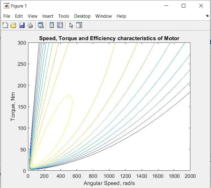
From this contour plot, we can see that the highest level of efficiency arises in the innermost contour plot and this efficiency decreases as the contours increase in size from the innermost contour.