Week-11 Challenge: Braking

Task-1

Braking: Braking is a function or force act to interrupt its actual condition. Here vehicle moving in certain speed (actual condition). Braking force or function acts on vehicle to interrupt its speed.

In simple words, the function of braking system is to bring the vehicle in to rest position or slow down from its actual speed.

Braking are two types 1. Electric braking(re-generative braking)

2. Mechanical braking

1.Electric braking:

In this type of braking, vehicle will generate the energy back to battery back, due to kinetic energy occurs during braking. These braking is possible by slow with long time. Then the efficiency of re-generative braking is high. The total generated Kinetic energy will collect back to storage.

2.mechanical braking:

In this type of braking, brakes are done at high, vehicle gets in to rest position in very small time. Here the friction force applied at brakes is high, the generated kinetic energy will be dissipated in the form of heat.

The kinetic energy of a vehicle during braking is

K.E = ½ * M*V^2

M is the mass of vehicle in Kg.

V is the velocity of vehicle in m/sec.

Here consider initial and final velocity.

Create a excel sheet of drive cycle

Consider vehicle mass is 1000 kg’s

MATLAB script file is created :

clc;

clear all;

% calculating the braking power = (1\2 * M*V^2)%

% braking energy = braking power / 3600%

M= 1000; %mass of vehicle%

num=xlsread('Drive cycle.xlsx'); %importing drive cycle file%

time=num(:,1); %time in sec%

velocity = num(:,2); %velocity in m/sec%

for i=1: (length(num)-1)

if velocity(i)>velocity(i+1)

Braking_energy(i)= 0.5*M*(((velocity(i) - velocity(i+1))^2))/3600; %energy required=0.5*M*V^2/3600%

end

end

fprintf('total brake energy is %d',sum(Breaking_energy))

%ploting

figure(1)

plot(time,velocity,'r--')

xlabel('time'); ylabel('velocity'); %labeling%

figure(2)

plot(Braking_energy,'g-')

xlabel('time'); ylabel('braking_energy'); %labeling%

Output:

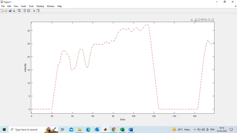
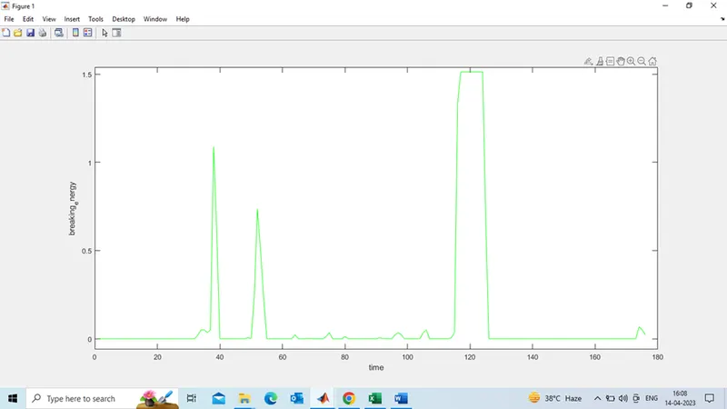
From the output, observed that braking curve figure(2) is reacted when the change in velocity in figure(1). At 120 sec velocity we can observe the very high braking, @5 sec. here kinetic energy is dissipated in the form of heat. Where as at small change in velocity at 40 sec, will get small brake likely to generate small amount of re-generative braking.

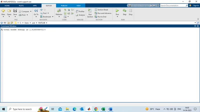
Here the total energy required for braking for considered drive cycle is 5.93 K.J.

Task-2:

The electric motor can’t develop the braking torque at high speed, similarly to starting because, when the supply is cut off to motor. It act as generator and produces kinetic energy due to moment of inertia. Here supply is cut off it results weaking of flux ,due to these effect motor can’t develop braking torque at high speed.

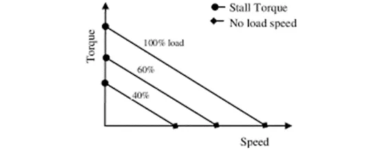
From the torque -speed characteristics we can observe that, at initial starting of motor have high torque at zero speed, by increasing of speed results decreases the torque. The braking function is observe in second quadrant operation. Here motor can’t develop braking torque at high speed like starting of motor.

Re-generative braking:

It is also called electric braking. These braking is applied by cut-off the supply to motor, then motor act as a generator( run in same direction until vehicle gets in to rest ). The time period between the supply cut-off and vehicle gets rest position is braking time. In regenerative braking vehicle takes more time to get into rest. In these case kinetic energy of vehicle runs the motor and generated energy feed back to the battery.

If the regenerative braking power requirement is more than the charging limit or more than the regenerative capacity of the machine we must apply the mechanical braking.

Mechanical braking have high braking efficiency but the vehicle efficiency may decreases due to elimination of re-generative braking ; kinetic energy is dissipated in the form of heat (wasted). And also friction applied on brakes is high, due to these friction brakes may warn out quickly.

To improve the braking efficiency and vehicle efficiency , the combined response of electric and mechanical braking is considered.

These combination can be achieved by two types of brake control strategies.

1. Series brake control strategy
2. Parallel brake control strategy

1.series brake control strategy:

This control strategy can be achieved by applying brakes one after another simultaneously. In these strategy we again divided based on comfort one is good comfort on braking and another one is energy efficiency. Here braking comfort may greatly possible by mechanical due to high efficiency and efficiency may be compromised.

2.parallel braking strategy:

This control strategy can be achieved by applying brakes of both electric and mechanical same time. With their level of percentage.

Here EDIB- electric driven intelligent brake is implement in vehicle to control brake strategy. Low speed braking have high efficiency of regenerative braking and high speed braking have combine braking.

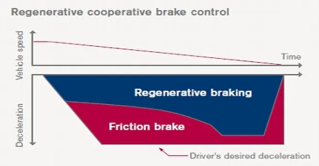
Here the combined braking control strategy implemented by control signal to both hydraulic brake or mechanical brake and re-generative brake or electric brake.

Task:3

The motor efficiency is mainly depends on its losses. The following types of losses are occurs in motor.

1. Copper losses(I^2 *R)
2. Iron losses
3. Windage losses
4. Constant losses

1.Copper losses: these losses are also called I^2 R losses. R is the armature resistance and I is the armature current which is directly proportional to torque.

I directly proportional to torque(T)

I= Kc* T

I^2 = Kc*T2

Copper losses = Kc*T^2

2.Iron losses: iron losses are nothing but magnetic losses. Where factor is based on magnetic effect. For permanent magnet have constant magnetic field and the iron losses are based on the value of speed. A various speed have different value of back emf. That are going to effect iron losses.

Iron losses =Ki*W (W is speed)

3.Windage losses: this is due to mechanical or friction of windage losses. These is based on size and shape of the motor.

Windage losses = Kw*W^3

4.Constant losses: these are constant at motor operation . which is denoted by ‘C’

Now the total losses = Copper losses + Iron losses+ Windage losses+ Constant losses

= Kc*T^2 + Ki*W+ Kw*W^3 +C

Total output power = torque *speed

Total input power = total output power + total losses.

Efficiency = Output power / input power

Contour plot: these plot represents the same height or three dimensional representation.

Matlab script is developed for contour plot of Speed, torque and efficiency

MATLAB script:

clear all

close all

clc

W = linspace(0,1000,300); %speed values%

T = linspace(0,250,300); %Torque values%

% motor constants%

Kc = 0.2; % Copper Loss constant

Ki = 0.008; % Iron Loss Constant

Kw = 0.0001; % Windage Loss Constant

Conl = 20; % Motor Loss Constant

%making mesh%

[X,Y] = meshgrid(W,T);

outputpower = X.*Y; % Calculating output power

B= ((Y.^2).*Kc); %Copper losses%

C= (Ki.*X); %Iron losses%

D=((X.^3).*Kw); %windage losses%

inputpower = outputpower + B + C +D +Conl; %total input power %

Z = outputpower./inputpower; %efficiency%

% set the effeiciency for contour plot%

V = [0.70,0.72,0.75,0.77,0.79,0.80,0.81,0.82,0.83,0.84,0.85,0.86,0.87,0.88,0.89,0.90,0.91,0.92,0.93,0.95];

contourf(X,Y,Z,V) %plotting%

xlabel('speed');ylabel('torque'); % labeling%

hold on;

V=[8000,10000];

contour(X,Y,outputpower,V); %Speed and torque curves%

title('Contour plot of efficiency and speed - torque curves')

OUTPUT:

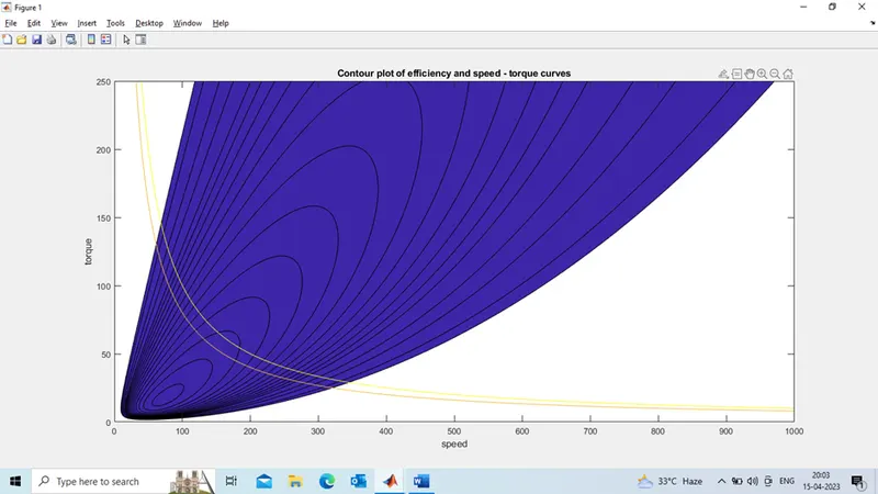
Here the output shows the contour plot of efficiency and speed- torque curves of a machine including losses.