Week-11 Challenge: Braking

Solution :

Q1) For a defined driving cycle, calculate the energy required for braking ?

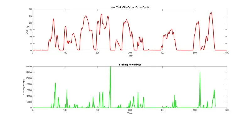
In this task a ' New York City Cycle' drive cycle is chose to calcualte the braking power for respective time period. Data is obtained from online platforms and put it all into excel sheet. A typical MATLAB program is built to obtain the power data of this cycle. All details are provided below,

MATLAB Code -

% For New york city cycle Drive cycle braking energy is calculated.
clc;
close all;
clear all;

%importing the excel file data of drive cycle.
drive_cycle = xlsread("NYCC Data.xlsx");
t =drive_cycle (:,1);                               % Time period data
v =drive_cycle (:,2);                               % Velocity data
m=800;                                              % Mass of vehicle in kgs

%Defining a loop with logic to calculate braking power enegry
for i=1:(length(drive_cycle) -1)
    if v(i)>v(i+1)
    B_power(i) = 0.5*m*(v(i)-v(i-1))^2;       % Formula for calculating braking power
    end
end
fprintf('Total brake enegry in watts is %d', sum(B_power)); % To print the total total braking energy in watt

figure(1)                               % Plotting the details of calculated parameters
subplot(2,1,1);
plot (t,v,'LineWidth',2,'color','r'); title('New York City Cycle - Drive Cycle')
ylabel ('Velocity');
xlabel('Time');

subplot(2,1,2);
plot (B_power,'linewidth',2,'color','g')
title('Braking Power Plot');
ylabel ('Braking enegry');
xlabel('Time');

Explanation of code -

• The NYCC drive cycle data is stored in excel file and read those data into matlab then read the separate values of time and velocity column wise.
• Fixing the value of vehicle mass as 800 kgs.
• Here a simple logic is developed to find out the braking power from the formula mentioned in code, the logic used is if the initial value of velocity is more than the next velocity then its braking region and loop will execute for only this condition by implementing the formula.
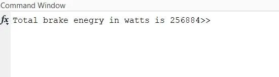
• After loop get executed for the logic developed then printing the sum of braking power in workspace window.
• a figure is plotted using the subplot commands and other detailing commands.

Output of code -

Workspace window

Conclution -

• For each braking period the braking power is calculated only and its shown in above figure by green color.
• Its Observed that the braking power is nothing but accelerating power but with negative polarity or magnitude.

(Note -Enclosed all files related to task.)

Ref - https://www.epa.gov/vehicle-and-fuel-emissions-testing/dynamometer-drive-schedules

Q2) Why electric motor can’t develop braking torque at high speed similar to starting? How electric and mechanical brakes are coordinated?

Whenever we talk about electric motors they are exceptional at propulsion whether it is AC motors or DC motors they have their own specialities of performance. As soon as the concer shifted to braking power or characteristics of these motor they left behind because the energy they omits while propulsion could not able to perform the same in braking operation.

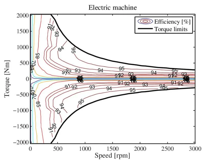
Braking torque of EV motors is not as high as accelerating torque, during the regeneratve braking mode it is not possible to get back aal the energy which was discharged. It might be due to complete reverse operation of its working which reduce its ability to perform in braking modes. Below fig represents the contour grapth of motor efficiency from it it can be observed that efficiency or torque points in motoring region is not same as in braking region ( negative torque).

To overcome above cons and to achieve a proper safe braking of EV below techniques are used -

1. Series Brakes :-

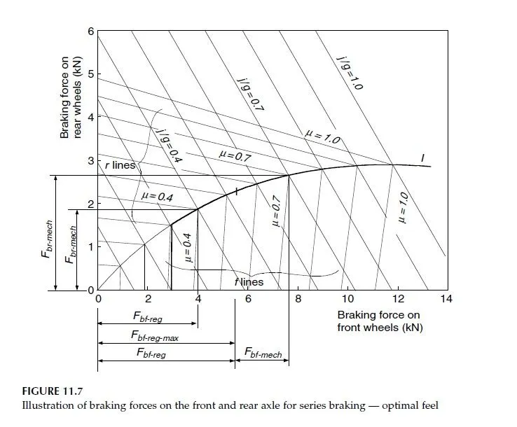
The series braking system with optimal feel consists of a braking controller that controls the braking forces on the front and rear wheels. The control objective is to minimize the stopping distance and optimize the driver’s feel. As mentioned in Section 2.9 of Chapter 2, the shortest braking distance and good braking feel require the braking forces on the front and rear wheels to follow the ideal braking force distribution curve I. Figure 11.7 illustrates the principle of this braking control strategy. When the commanded deceleration (represented by the braking pedal position) is less than 0.2 g, only the regenerative braking on the front wheels is applied, which emulates the engine retarding function in conventional vehicles. When the commanded deceleration is greater than 0.2 g, the braking forces on the front and rear wheels follow the ideal braking forces distribution curve I, as shown in Figure 11.7 by the thick solid line. The braking force on the front wheels (driven axle) is divided into two parts: regenerative braking force and mechanically frictional braking force. When the braking force demanded is less than the maximum braking force that the electric motor can produce, only electrically regenerative braking will apply. When the commanded braking force is greater than the available regenerative braking force, the electric motor will operate to produce its maximum braking torque, and the remaining braking force is met by the mechanical brake system.

It should be noted that the maximum regenerative braking force produced by an electric motor is closely related to the electric motor’s speed. At low speed (lower than its base speed), the maximum torque is constant. However, at high speed (higher than its base speed), the maximum torque decreases hyperbolically with its speed. Therefore, the mechanical brake torque at a given vehicle deceleration varies with vehicle speed.

2. Parallel Brakes :-

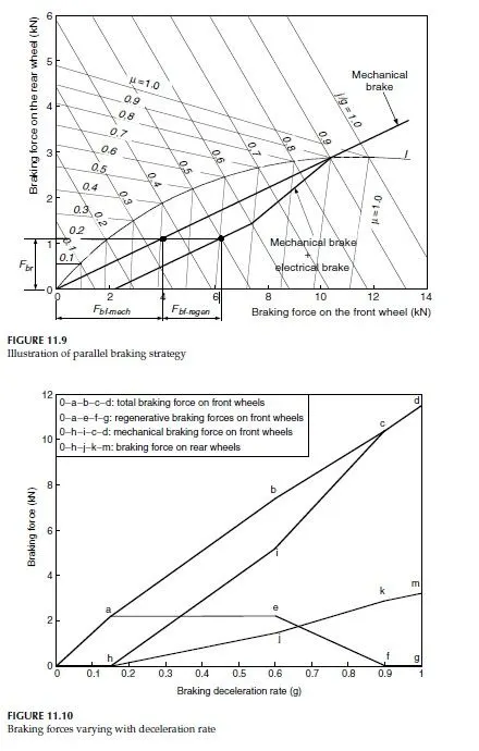
The parallel brake system includes both an electrical (regenerative) brake and a mechanical brake, which produce braking forces is parallel and simultaneously. The operating principle is illustrated in Figure 11.9, in which regenerative braking is applied only to the front wheels. The parallel brake system has a conventional mechanical brake which has a fixed ratio of braking force distribution on the front and rear wheels.
Regenerative braking adds additional braking force to the front wheels, resulting in the total braking force distribution curve. The mechanical braking forces on the front and rear axles are proportional to the hydraulic pressure in the master cylinder. The regenerative braking force developed by the electric motor is a function of the hydraulic pressure of the master cylinder, and therefore a function of vehicle deceleration. Because the regenerative braking force available is a function of motor speed and because almost no kinetic energy can be recovered at low motor speed, the regenerative braking force at high vehicle deceleration (e.g., a/g0.9) is designed to be zero so as to maintain braking balance. When the demanded deceleration is less than this deceleration, regenerative braking is effective. When the braking deceleration commanded is less than a given value, say 0.15 g, only regenerative braking is applied. This emulates the engine retarding in a conventional vehicle. In Figure 11.9, the regenerative braking force, Fbf-regen, and mechanical braking forces on the front and rear wheels, Fbf-mech and Fbr, are illustrated. Figure 11.10 shows the total braking force, regenerative braking force, and mechanical braking force on the front wheels as well as the braking force on the rear wheels in the parallel braking system of a passenger car.

The parallel braking system does not need an electronically controlled mechanical brake system. Apressure sensor senses the hydraulic pressure in the master cylinder, which represents the deceleration demand. The pressure signal is regulated and sent to the electric motor controller to control the electric motor to produce the demanded braking torque. Compared with the series braking of both optimal feel and energy recovery, the parallel braking system has a much simpler construction and control system.4 However, the driver’s feeling, and amount of energy recovered are compromised.

Ref -

• Modern electric, hybrid electric and fuel cell vehicles – Fundamentals, Theory and Design. By Mehrdad Ehsani, Yimin Gao, Sebastien E Gay, Ali Emadi. CRC Press 2005

• https://www.researchgate.net/figure/The-efficiency-of-the-electric-motor-as-a-function-of-the-torque-and-speed-For-positive_fig1_320565225

Q3) Make a MATLAB program which plots contour of given motor speed, torque and efficiency values. Attach the code as a .m file attach a screenshot of all the plots.

Contour Plots :

A contour plot is a graphical technique for representing a 3-dimensional surface by plotting constant z slices, called contours, on a 2-dimensional format. That is, given a value for z, lines are drawn for connecting the (x,y) coordinates where that z value occurs.

Contour plots display the results of a single data set (time step, load step, or substep) over the model geometry. The range of values in the results set is divided into a number of subranges (nine by default), and each subrange is assigned a color. The colors are then mapped over the geometry to indicate the result values at each location in the model. Most results for continuum (e.g., PLANE and SOLID) elements can be displayed as contour plots. For beam and shell elements, it may be necessary to issue the /ESHAPE command before creating a contour plot or to plot the results using element tables instead.

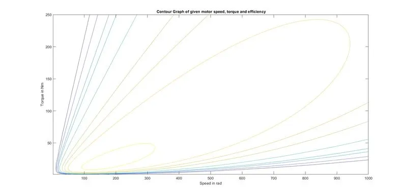
To plot the contour graph of motor along with its speed torque and efficiency values a MATLAB program is developed which is provided below. The standard values of copper loss , iron loss, windage loss & constant are taken.

MATLAB Program -

% For ploting contour of given motor speed, torque and efficiency values.

clc;
clear all;
close all;
x= linspace (1,1000);  % defining array in x axis for speed.
y= linspace (1,250);   % y axis for torque T

%defining motor loss constants.
kc=0.2;              % For Copper loss in motor
ki=0.008;            % For Iron loss
kw= 0.00001;         % For windage loss
ConL = 20;           % Constant motor losses

% Now Creating a mesh for plotting 
[X,Y]=meshgrid(x,y);
outputpower= (X.*Y);  % POwer = torque x speed
B=(Y.^2)*kc;          % Copper loss 
C= X.*ki;             % Iron loss
D=(X.^3)*kw;          % Windage loss
Inputpower = outputpower+B+C+D+ConL;
Z= outputpower./Inputpower;

% setting the efficiency range 
V= [0.70, 0.74 ,0.78, 0.80, 0.84, 0.88, 0.90, 0.92, 0.95];
box off
grid off
contour(X,Y,Z,V);
xlabel('Speed in rad');
ylabel ('Torque in Nm');
title(' Contour Graph of given motor speed, torque and efficiency')

Output of code -

Conclusion -

• Using the developed logic the contour grapth is successfully plotted for the motor speed, torque and efficiency values.
• Contour Graph is a 2D representation of 3D values , the smallest circular area is highest efficiency point and largest one is smallest efficiency point.

Reference -

• https://www.researchgate.net/figure/The-efficiency-of-the-electric-motor-as-a-function-of-the-torque-and-speed-For-positive_fig1_320565225
• https://www.itl.nist.gov/div898/handbook/eda/section3/contour.htm#:~:text=A%20contour%20plot%20is%20a,where%20that%20z%20value%20occurs.