Braking Calculation
Objective:
- To define a drive cycle and calculate the braking energy required.
- To define why electric vehicles cannot generate braking torque at high speed compared to starting and also state how electric vehicles are coordinated.
- To create a Matlab code that plots contour of given motor speed, torque, and efficiency values.
Objective-1:
First, we will have to create a Drive cycle and note the places where the braking is done and also the change in speed in those regions.
Here is a link for the Drive cycle and Brake energy calculation excel sheet.
https://docs.google.com/spreadsheets/d/1OHxl4mx1kSFZSZwwGrP1B86vsWlrWt5NOTgsAu3kwmY/edit?usp=sharing
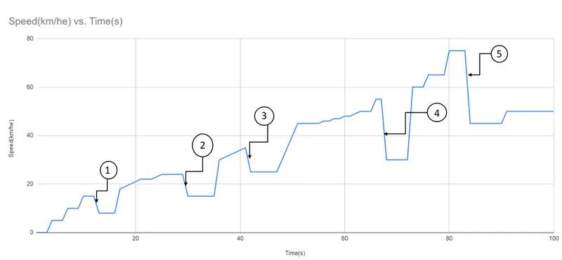
From the above drive cycle graph, we can see that the braking is done 5 times. So we will be calculating the Energy needed for each instance and will be adding them to find the total Brake energy.
Kinetic Energy=`frac{1}{2}mxxv^2`
m=mass od the vehicle
v=velocity of the vehicle( Also it can be (Initial Velocity- Final velocity)for some scenarios)
Below is the image showing the calculation done to find the braking energy.
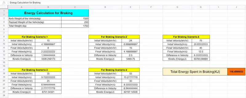
From the above image, you can see that the Total Braking Energy has been calculated for the Given drive cycle.
Objective-2:
Mechanical Braking:
Mechanical brakes all act by generating frictional forces as two surfaces rub against each other. The stopping power or capacity of a brake depends largely on the surface area of frictional surfaces as well as on the actuation force applied. The friction and wear encountered by the working surfaces are severe. Thus, the durability of a brake or service life between maintenance depends heavily on the type of material used to line the shoe or pad.
Electric Braking:
- Series Control Strategy
- Parallel Control Strategy
Series Control Strategy:
- a combination of a friction-based mechanical braking system with a regenerative braking system that transfers energy to the battery with integrated control, which distributes the required braking force between the regenerative braking system and the mechanical braking system.
- Series Strategy could give an increase of 15-30% in fuel efficiency and has more consistent braking due to good torque blending capability.
Parallel Control Strategy:
- Combination of mechanical and the regenerative braking system operated simultaneously without an integrated control.
- The regenerative braking force is added to the mechanical braking force which cannot be controlled.
- The regenerative torque is determined by considering the motor capacity, battery SOC, and vehicle velocity. The regenerative braking force is calculated from the brake control unit by comparing the demanded brake torque and the motor torque available.
At low speed, the Control unit usually uses Regenerative braking, and while when the vehicle is moving at high speeds the vehicle uses both Mechanical and Regenerative braking to slow down the vehicles.
Objective-3:
We will be creating a Matlab code to plot the Efficiency of a Motor.
In order to plot the efficiency, we first will be stating the losses that occur in a Motor.
Windage Loss:
Windage is a force created on an object by friction when there is relative movement between air and the object. Windage loss is the reduction in efficiency due to windage forces.
For example, electric motors are affected by friction between the rotor and air. Large alternators have significant losses due to windage. To reduce losses, hydrogen gas may be used, since it is less dense.
There are two causes of windage:
- The object is moving and being slowed by resistance from the air.
- A wind is blowing producing a force on the object.
Windage Loss= `K_wxxW^3`
Copper Loss:
Copper loss refers to a loss occurring due to the electrical resistance of current flowing through a winding (coil).
Iron Loss:
clear all
close all
clc

%Torque Inputs(N/m)
T=linspace(0,250);

%Speed values(rad/s)
W=linspace(0,1000);

%Meshgrid
[X Y]=meshgrid(W,T);%Loss Coefficients
Copper=0.17; %Copper Coefficient
Iron=0.006; %Iron Coefficient
Windage=0.000015; %Windage Coefficient
%Losses
Copper_Loss=Copper*(Y.^2); %Copper Losses
Iron_Loss=Iron*(X.^2); %Iron Losses
Windage_Loss=Windage*(X.^3); %Windage Losses
Con1=18; %Constant Motor LossSo now we will be providing the required Coefficients and will be calculating the Copper loss, Iron loss, Windage loss and Constant motor loss.
%Output Power
Power_Output=(X.*Y);
%Input Power
Power_Input=Power_Output+Copper_Loss+Iron_Loss+Windage_Loss+Con1;We will be calculating the Input and Output Power using the above code. You can see that Power input is the sum of Output power and the losses.
%Efficiency
Efficiency=Power_Output./Power_Input;The Efficiency of the motor is given by Output power and Input power.
%Efficiency values for contour
w=linspace(0.75,0.95,7);
%Contour Plot
contourf(X,Y,Efficiency,w,'showtext','on')
colorbar
grid on
xlabel('Angular Speed,rad/s')
ylabel('Torque,Nm')
title('Speed, Torque and Efficiency characteristics of Motor')We will be providing the above code to plot the results that we have obtained.
Full Matlab Code:
clear all
close all
clc
%Torque Inputs(N/m)
T=linspace(0,250);
%Speed values(rad/s)
W=linspace(0,1000);
%Meshgrid
[X Y]=meshgrid(W,T);
%Loss Coefficients
Copper=0.17;      %Copper Coefficient
Iron=0.006;       %Iron Coefficient
Windage=0.000015; %Windage Coefficient

%Losses
Copper_Loss=Copper*(Y.^2);       %Copper Losses
Iron_Loss=Iron*(X.^2);           %Iron Losses
Windage_Loss=Windage*(X.^3);     %Windage Losses
Con1=18;              %Constant Motor Loss
%Output Power
Power_Output=(X.*Y);
%Input Power
Power_Input=Power_Output+Copper_Loss+Iron_Loss+Windage_Loss+Con1;
%Efficiency
Efficiency=Power_Output./Power_Input;
%Efficiency values for contour
w=linspace(0.75,0.95,7);

%Contour Plot
contourf(X,Y,Efficiency,w,'showtext','on')
colorbar
grid on
xlabel('Angular Speed,rad/s')
ylabel('Torque,Nm')
title('Speed, Torque and Efficiency characteristics of Motor')Graph:
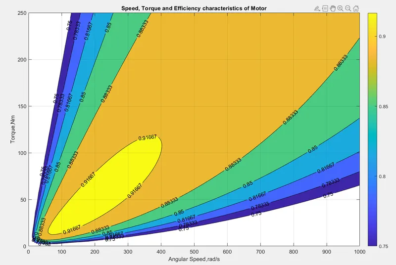
You can see the above graph with Speed on the x-axis and Torque on y-axis and the color bar represents the efficiency.