Week-11 Challenge: Braking
- For a defined driving cycle, calculate the energy required for braking.
sol: For this problem, UDDS drive cycle is considered. The UDDS drive cycle figure is given below:
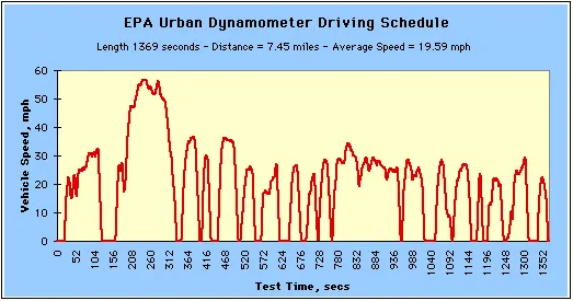
By using an excel sheet the drive cycle is uploaded into Matlab. The corresponding excel sheet is attached.
By using Matlab code the braking energy is calculated.
The formula for the braking energy is 1/2mV^2.
clc;
clear all;
m=2400;
DC_1 = xlsread('UDDS.xlsx');
v=DC_1( :,2);
t=DC_1( :,1);
v_ms = v *(1609.34/3600);
for i=1:1369
    if v_ms(i)>v_ms(i+1)
       BE(i)= (0.5*m*(v_ms(i)-v_ms(i+1))^2)/1000;    %Energy kwh%
    end
end
Breaking_Energy= mean(BE);
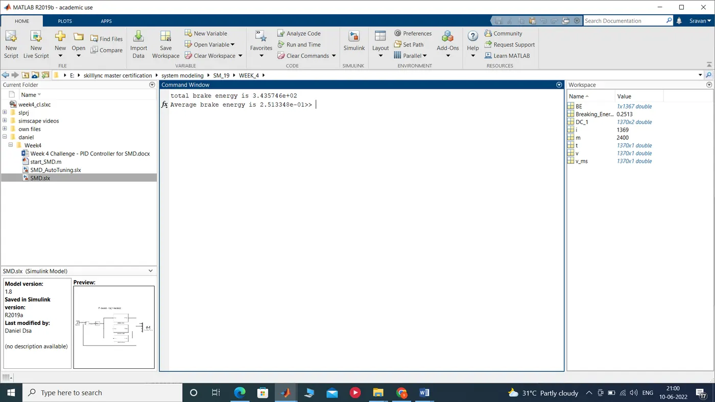
fprintf('total brake energy is %d\n', sum(BE))
fprintf('Average brake energy is %d', Breaking_Energy)

figure(1)
subplot(2,1,1)
plot(t,v,'r')
grid on
xlabel('time(Sec)')
ylabel('Velocity(mph)')
title('UDDS_Drive_Cycle')

hold on
subplot(2,1,2)
plot(t(1:1367),BE,'blue')
grid on
xlabel('time(Sec)')
ylabel('Energy_KWH')
title('Regenerative Breaking(kwh)')
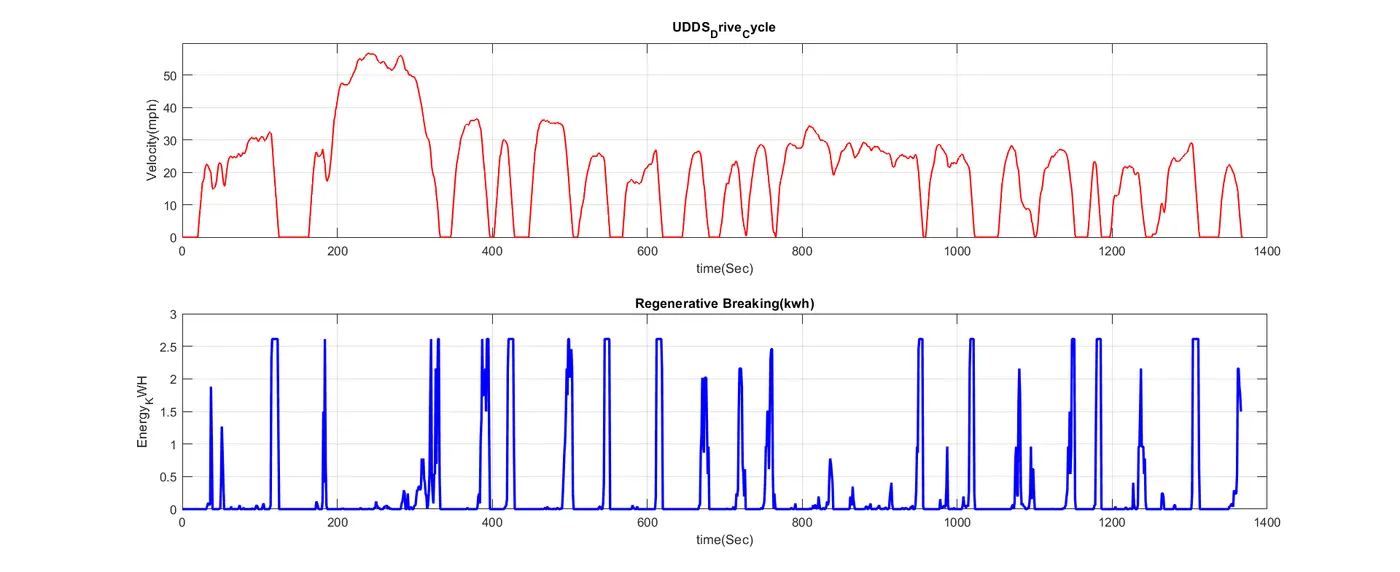
From the above graph, it is clear that the braking energy is present only when the vehicle is in a deceleration period.
2. Why electric motor can’t develop braking torque at a high speed similar to starting? How electric and mechanical brakes are coordinated?
The electric motor can't develop braking torque at a high speed similar to starting, because Braking torque is applied in the opposite direction of the rotation. We can use a mechanical brake to produce a braking torque.
Also as per the concept at starting or very low speeds the torque is very higher. In the deceleration period, the speed is higher than that of the acceleration period hence the braking torque is less.
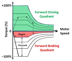
The coordination between electrical and mechanical brakes depends upon the braking we used. Generally, regenerative braking is used in traction. when the mechanical brakes have been applied the power from the source is very less and the motor acts as a generator due to its kinetic energy. Now the power is fed back to supply and In INDIA Shatabdi and Rajadhani trains are used regenerative braking, From this nearly 11 to 12% of energy is saved.
3.Make a MATLAB program which plots contour of given motor speed, torque and efficiency values. Attach the code as a .m file and attach a screenshot of all the plots.
%Make a MATLAB program which plots contour of given motor speed, torque
%and efficiency values.
%Attach the code as a .m file attach a screenshot of all the plots.
%--------------------------------------------------------------------%
x=linspace(1,1000);     %speed in terms of rad/sec.
y=linspace(1,250);      %Torque in terms of Nm.

%kc,ki,kw and CL values
kc=0.2;                %Constant for Copper losses.
ki=0.0008;               %Constant for iron losses.
kw=0.00001;             %Constant for Windage losses.
CL=20;                  %Constant Losses.
[X,Y]= meshgrid(x,y);   %To plot contour meshgrid is used.
OP=(X.*Y);              %Output Power= speed*Torque
CU_L=((Y.^2)*kc);       %Copper_losses
IL=(X*ki);              %Iron_Losses
WL=((X.^3)*kw);         %Windage_Losses.
IP=OP+CU_L+IL+WL+CL;    %Input Power= Outputpower+Losses.
Z=OP./IP;               %Efficiency
contour(X,Y,Z,5);
title('Efficiency contour for EM')
xlabel('speed in rad/sec')
ylabel('Torque in N-m')
hold on
P=[5000,10000];         %contours at 5kw and 10kw
contour(X,Y,OP,P);
Results:
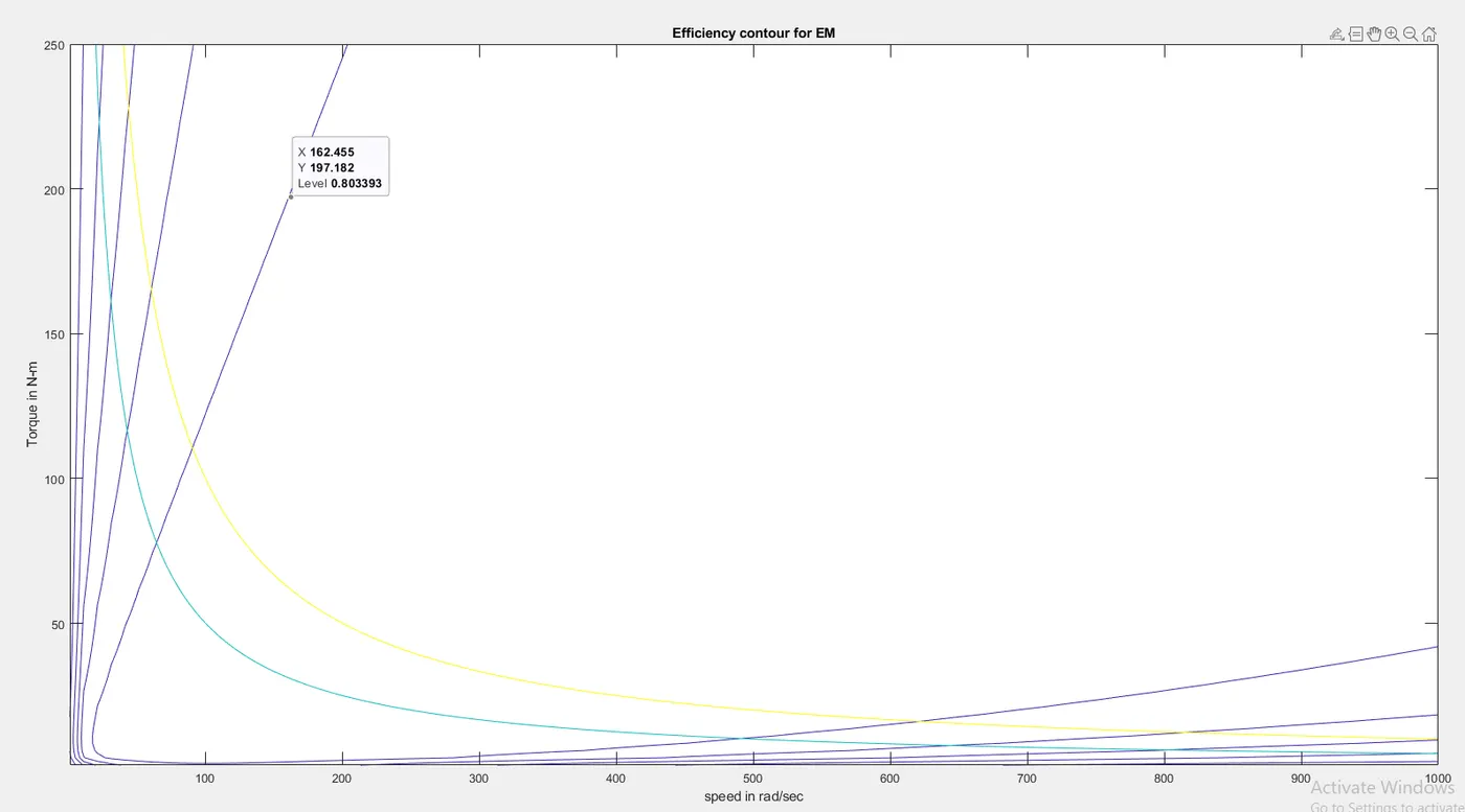
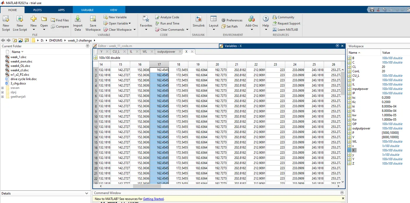
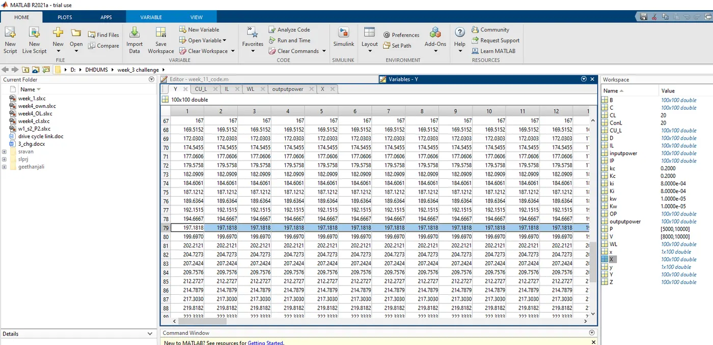
X=162.455 y=197.182.
The corresponding workspace blocks are shown in the below figures.
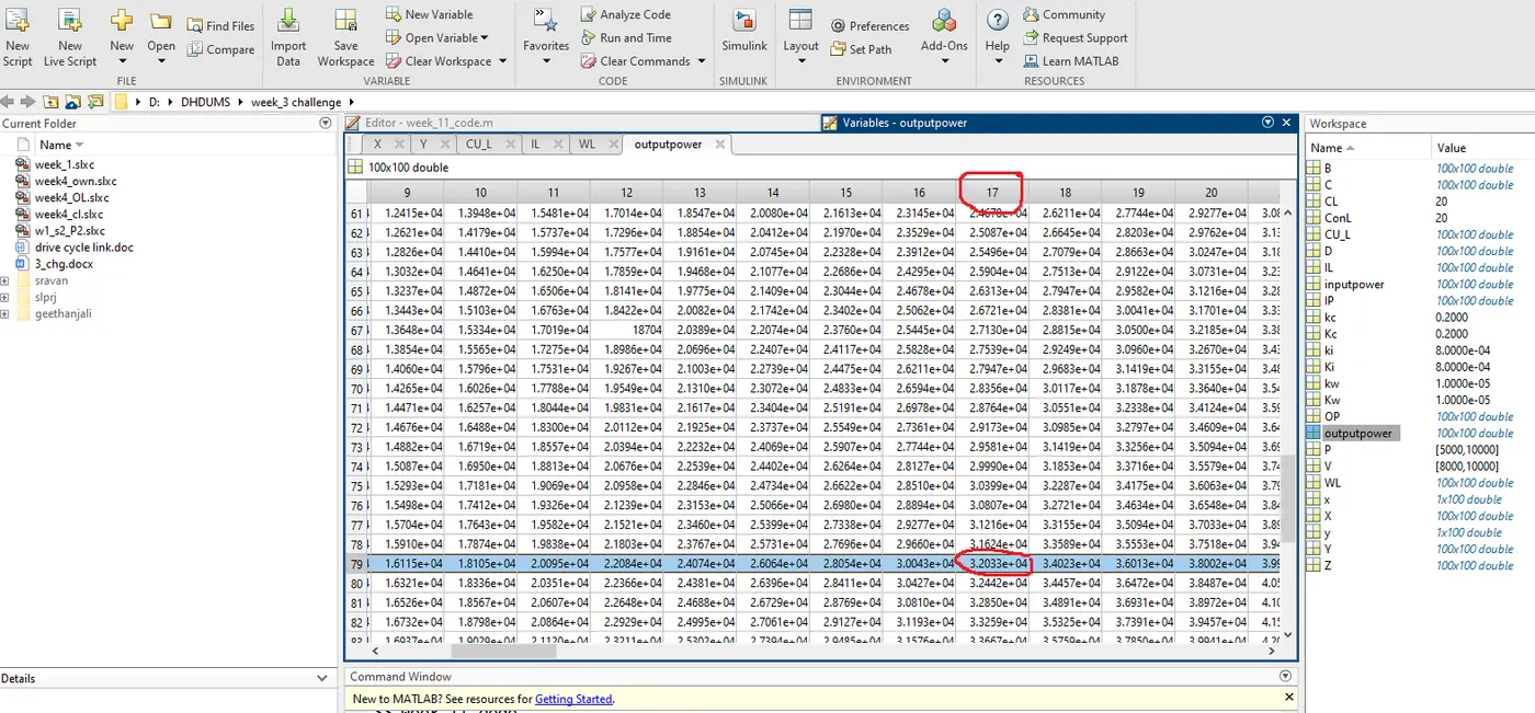
Output power validation=x*y
=162.455*197.182
=3.2*10^4;
The corresponding workspace variable is shown in the below figure.
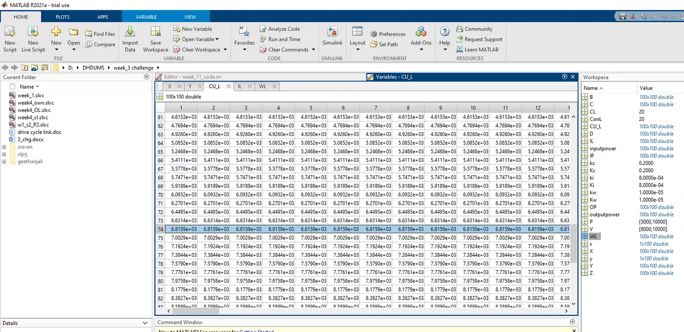
Copper loss= kc*y^2
= 0.2*184.6^2.
= 6.815*10^3.
The corresponding workspace variable is as shown in the below figure.
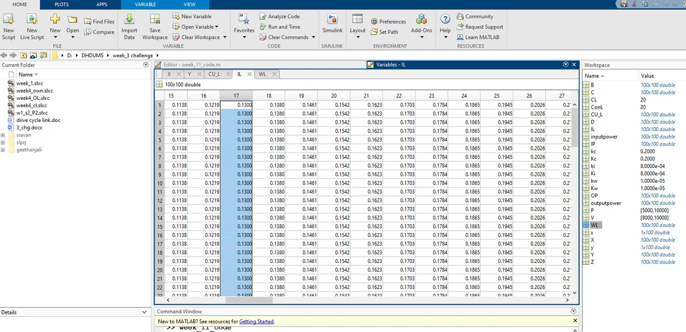
Iron loss= ki*x
= 0.0008*162.455
= 0.1299
The corresponding workspace variable is as shown in the below figure.
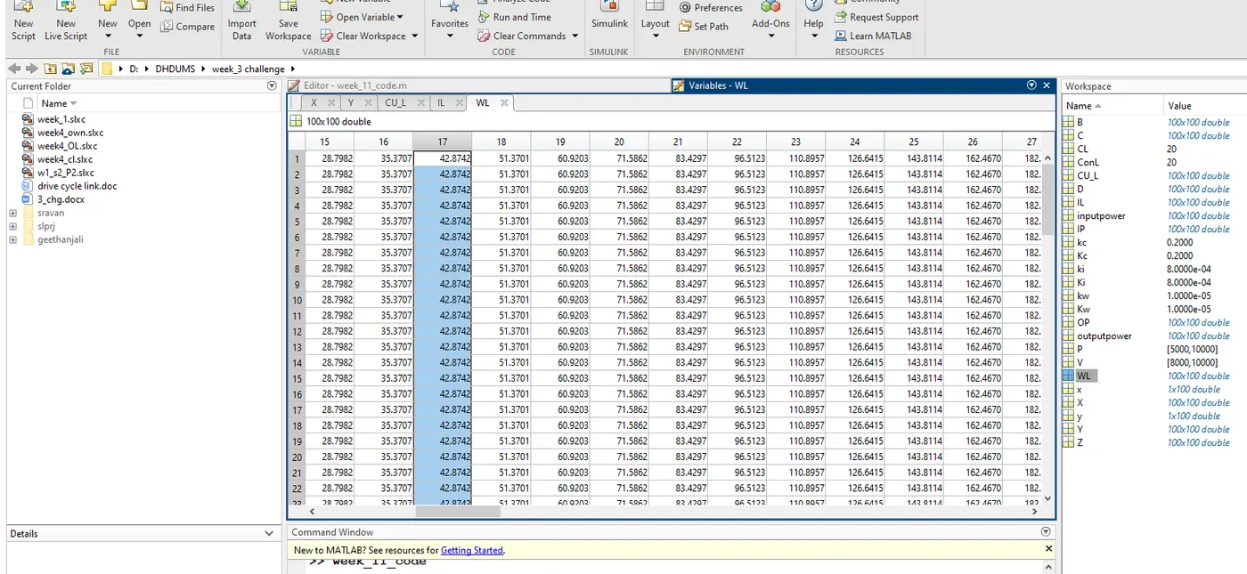
Windage loss= x.^3*kw
=162.45^3*0.00001
=42.8
The corresponding workspace variable is as shown in the below figure.
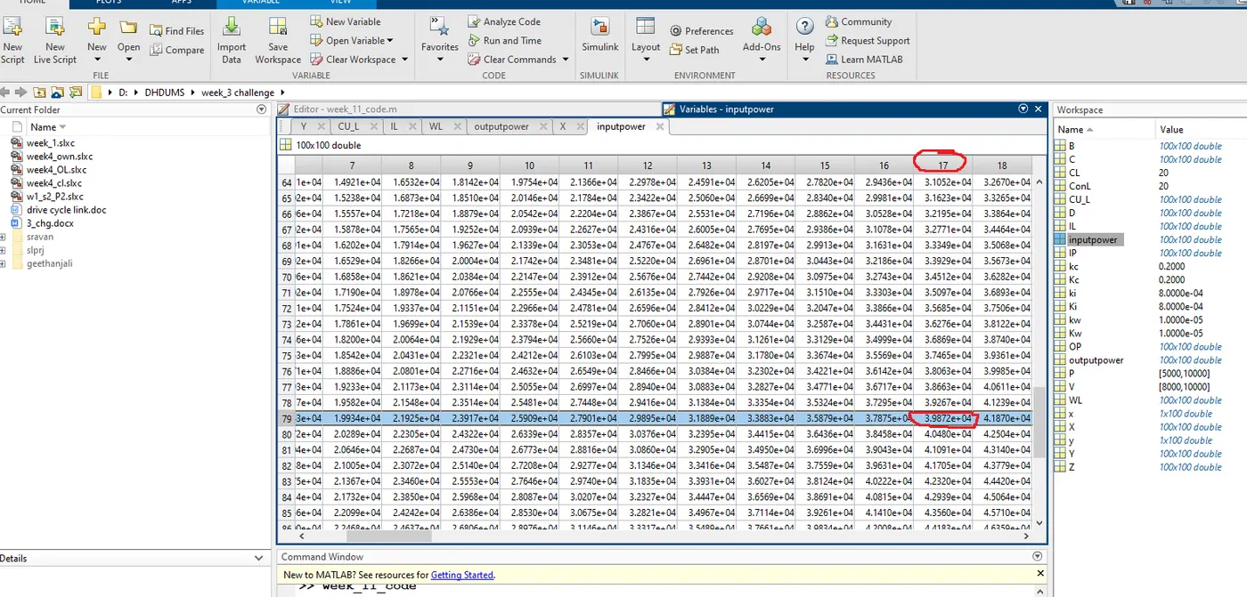
Input power= Output power+cu_l+w_l+I_l+cl
= (3.2*10^4)+(6.815*10^3)+42.8742+0.1299+20
=3.88*10^4;
The corresponding workspace variable is as shown in the below figure.
Z= op/ip
=(3.2*10^4)/(3.98*10^4)
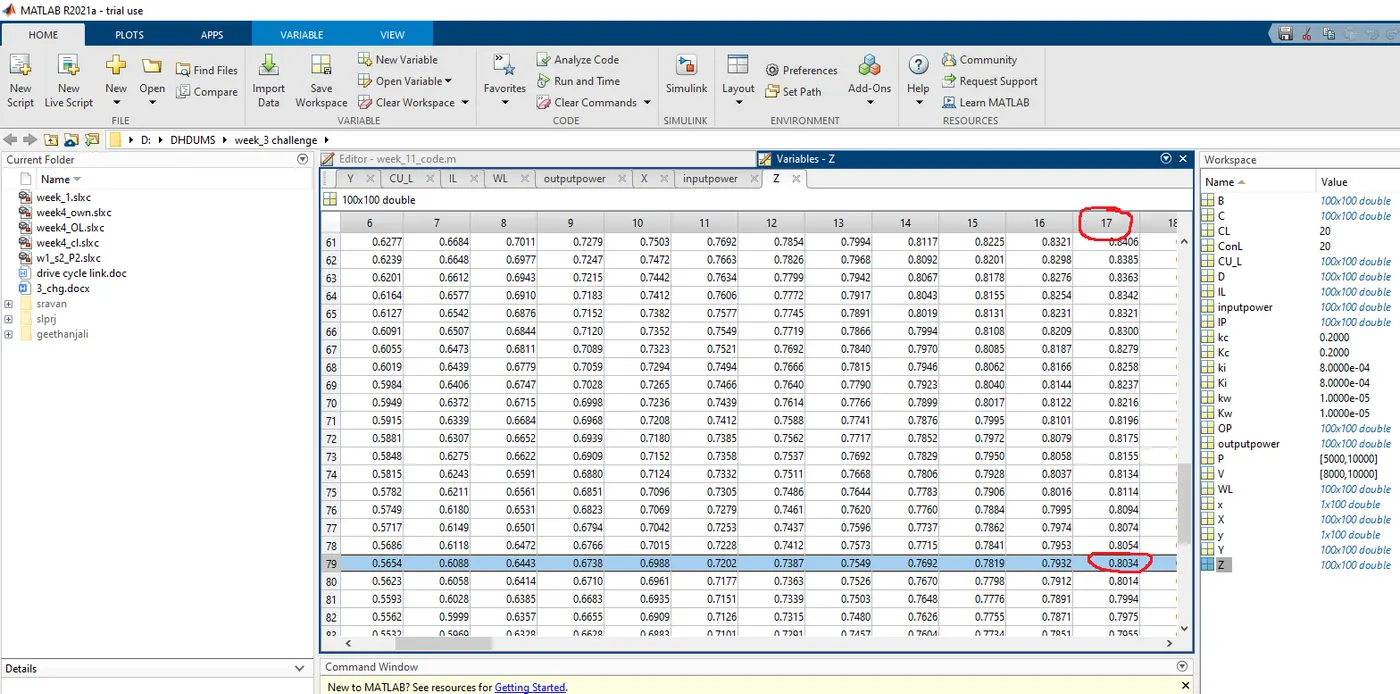
=0.8
The corresponding workspace variable is as shown in the below figure and the same is displayed in contour plot.
The output power contour with the 5kw range is as shown in figure below
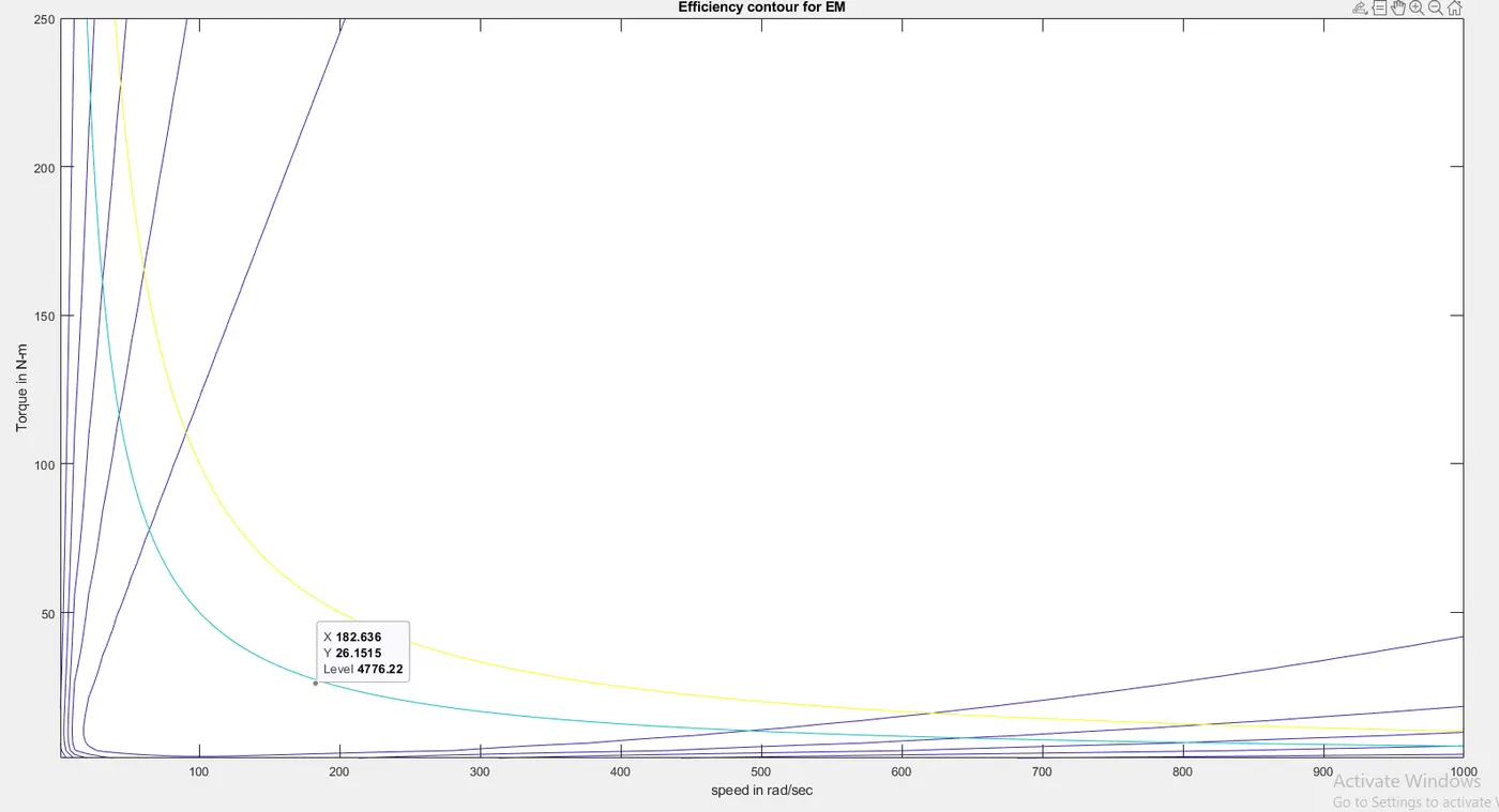
Consider the x and y values shown above and we will find the output power(level)
X=182.636 AND Y=26.15
Output power = x.*y
=182.636*26.15
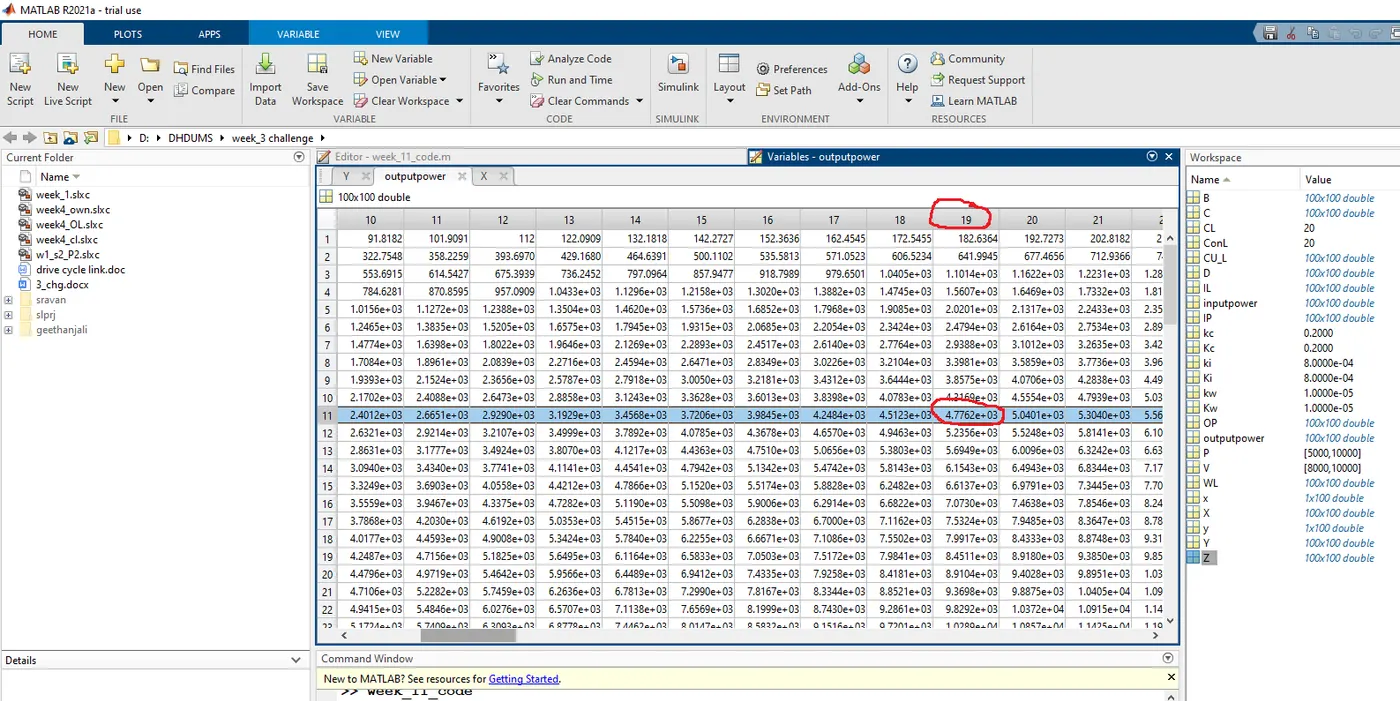
=4.776*10^3;
The corresponding workspace variable is as shown in the below figure.
From the above contour graphs it is observed that curves are not properly distributed. Hence here we will take efficieny vector so that it will plot with in the range only.The corresponding code is below:
%Make a MATLAB program which plots contour of given motor speed, torque
%and efficiency values.
%Attach the code as a .m file attach a screenshot of all the plots.
%--------------------------------------------------------------------%
x=linspace(1,1000);     %speed in terms of rad/sec.
y=linspace(1,250);      %Torque in terms of Nm.

%kc,ki,kw and CL values
kc=0.2;                %Constant for Copper losses.
ki=0.0008;               %Constant for iron losses.
kw=0.00001;             %Constant for Windage losses.
CL=20;                  %Constant Losses.
[X,Y]= meshgrid(x,y);   %To plot contour meshgrid is used.
OP=(X.*Y);              %Output Power= speed*Torque
CU_L=((Y.^2)*kc);       %Copper_losses
IL=(X*ki);              %Iron_Losses
WL=((X.^3)*kw);         %Windage_Losses.
IP=OP+CU_L+IL+WL+CL;    %Input Power= Outputpower+Losses.
Z=OP./IP;               %Efficiency
V = [0.70,0.80,0.85,0.90,0.91,0.92,0.925,0.93];
contour(X,Y,Z,V);
title('Efficiency contour for EM')
xlabel('speed in rad/sec')
ylabel('Torque in N-m')
hold on
P=[5000,10000];         %contours at 5kw and 10kw
contour(X,Y,OP,P);
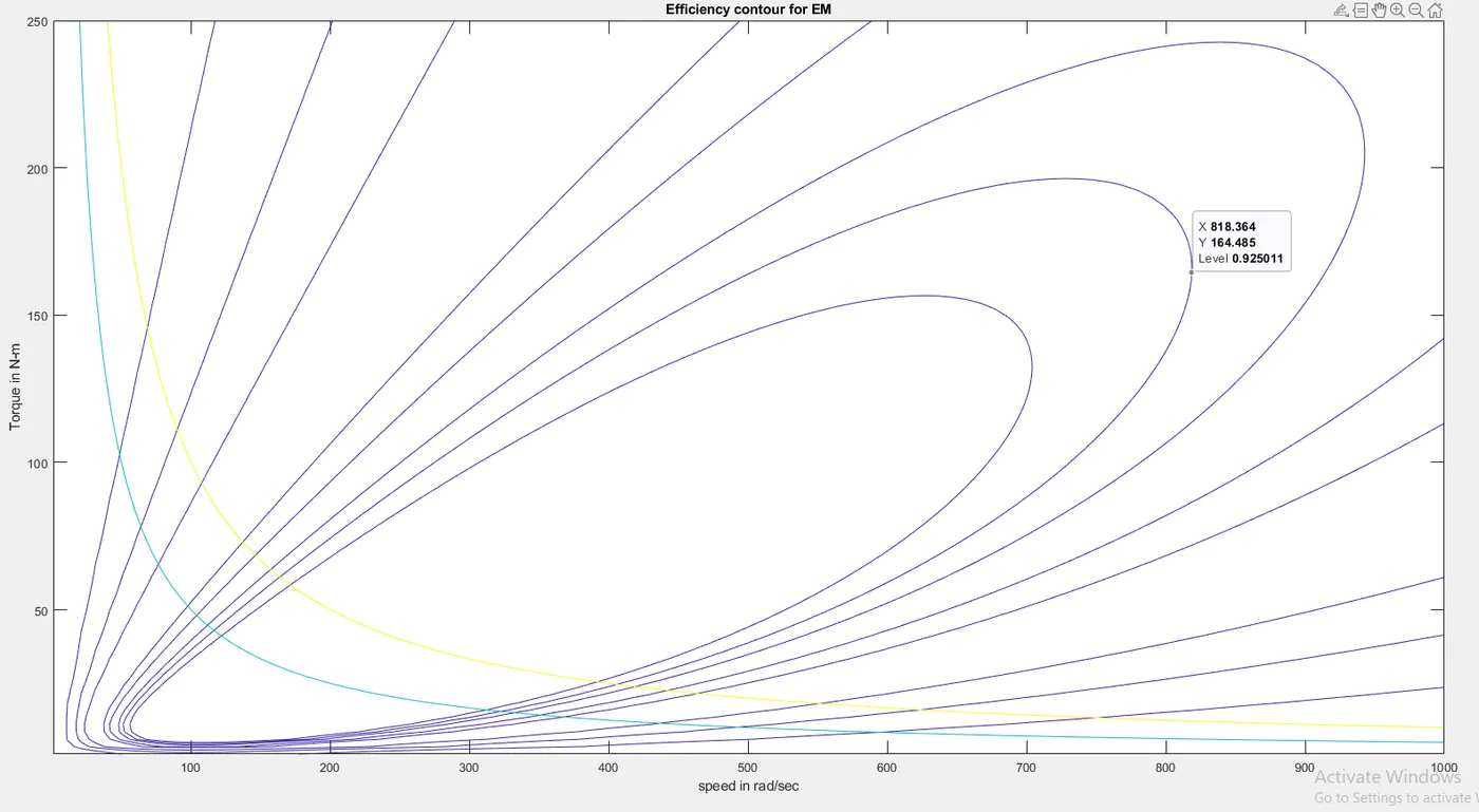
V = [0.70,0.80,0.85,0.90,0.91,0.92,0.925,0.93];
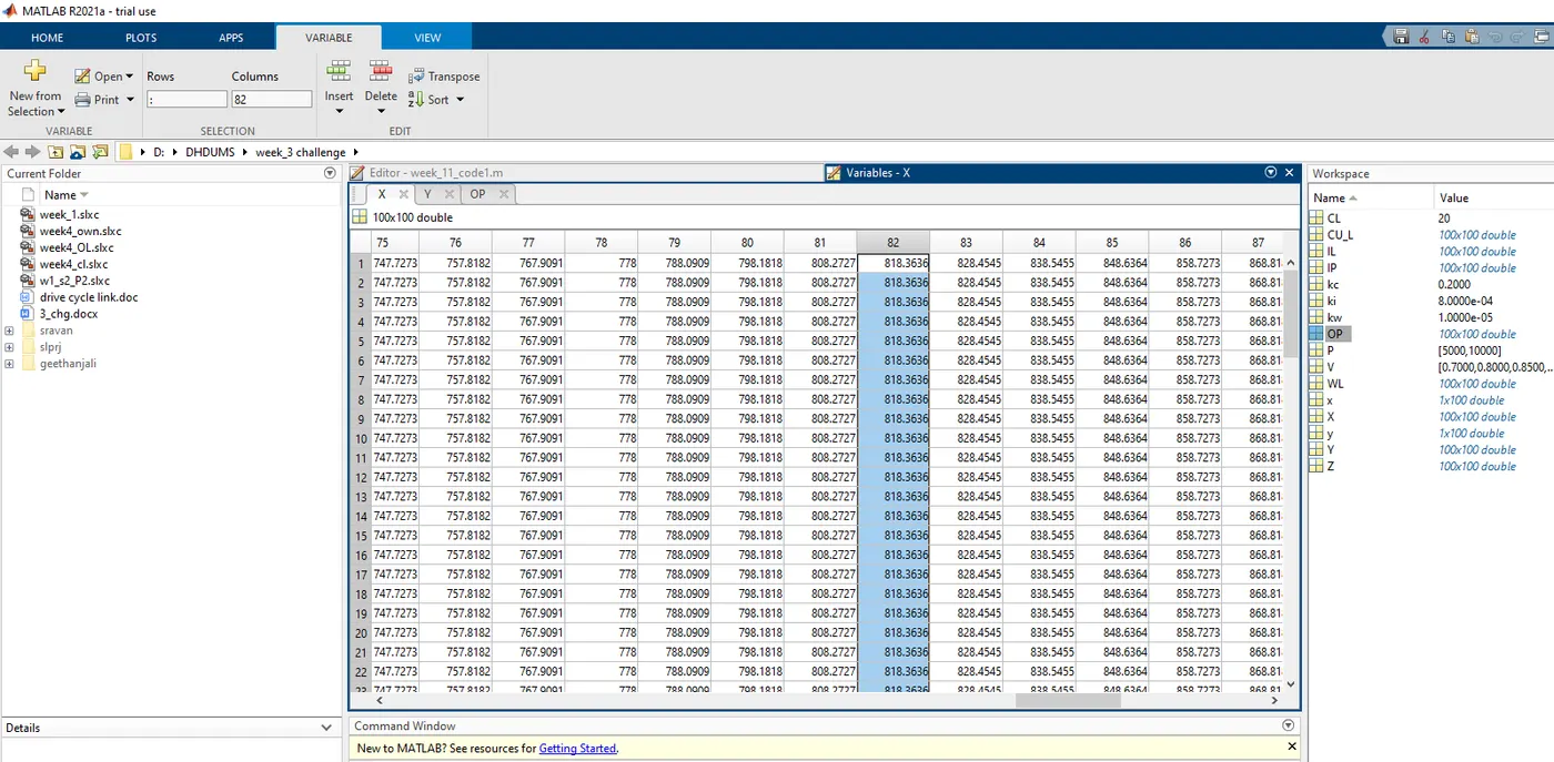
As per this vector, the above graph shows x=818.364 and y=164.485 values and the corresponding efficiency is 92.5(level).
x=818.364
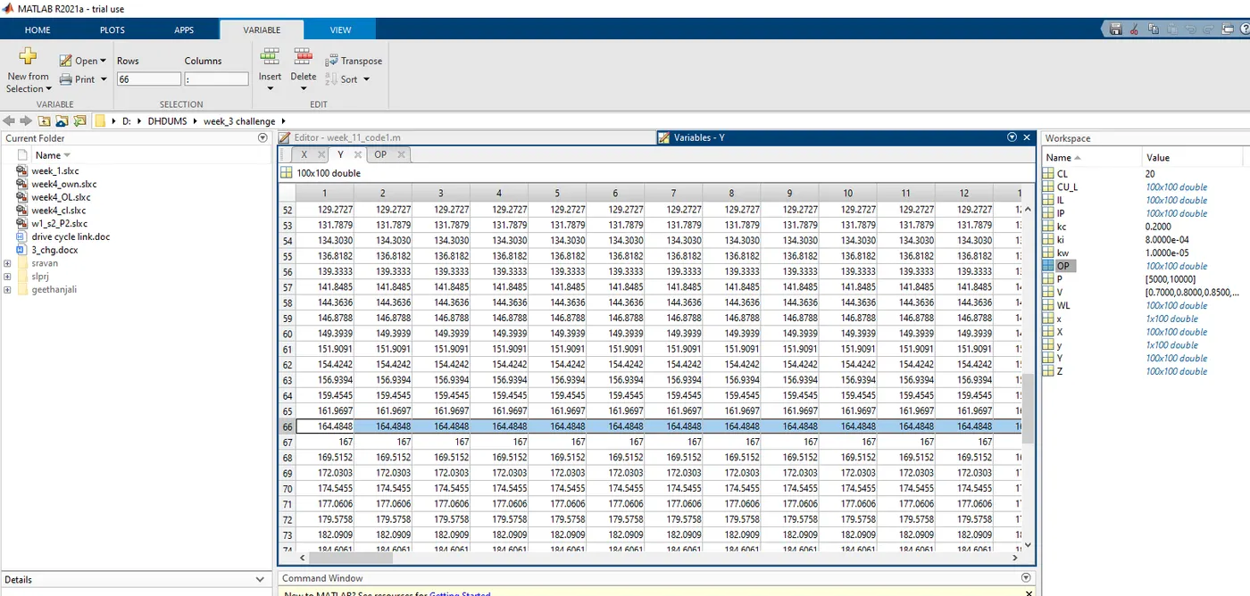
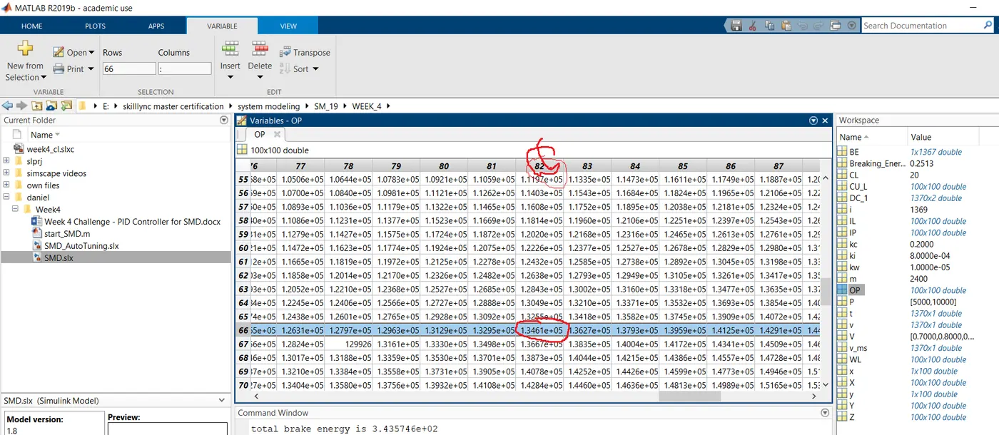
Output power =x*y
=818.364*164.485
=1.346*10^5;
The corresponding workspace variable is as shown in the below figure.
Copper loss= kc*y^2
= 0.2*164.485^2.
= 5.411*10^3.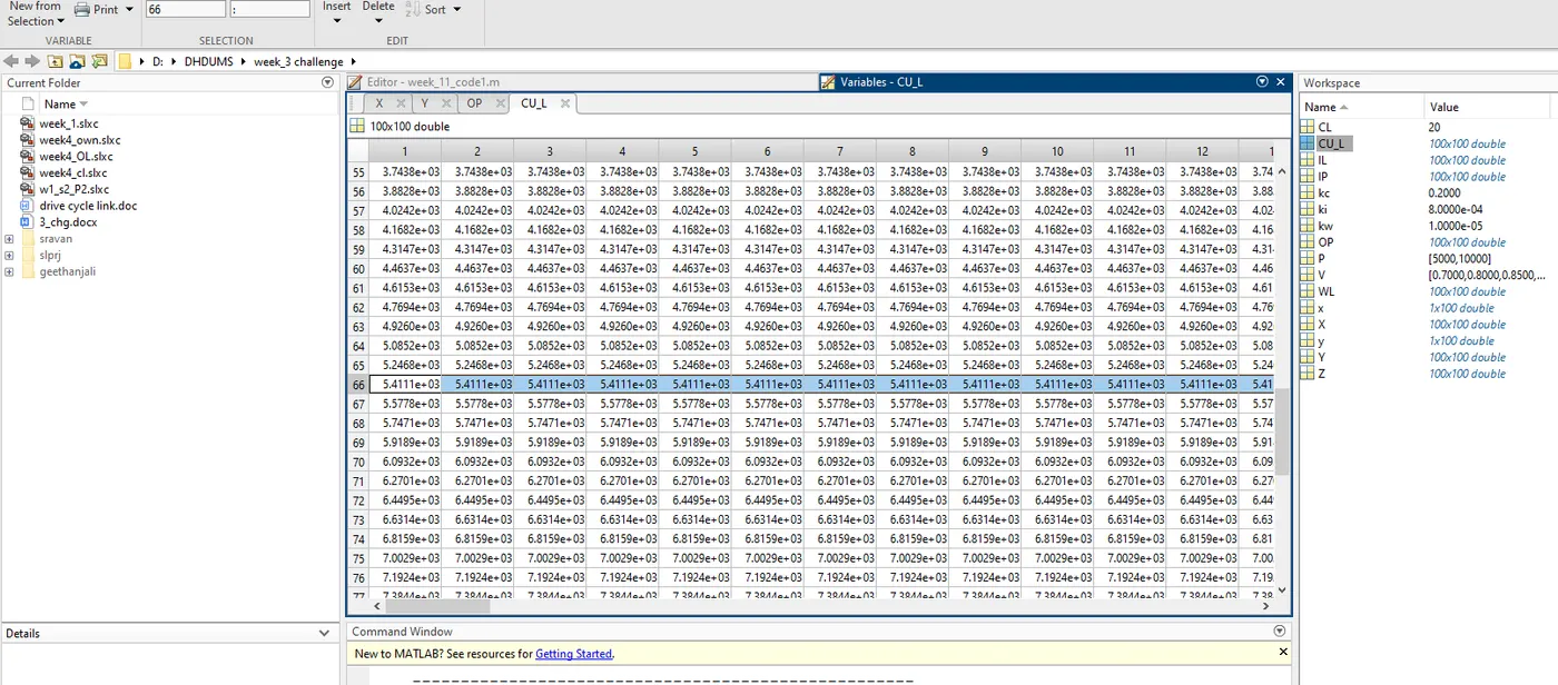
Iron loss= ki*x
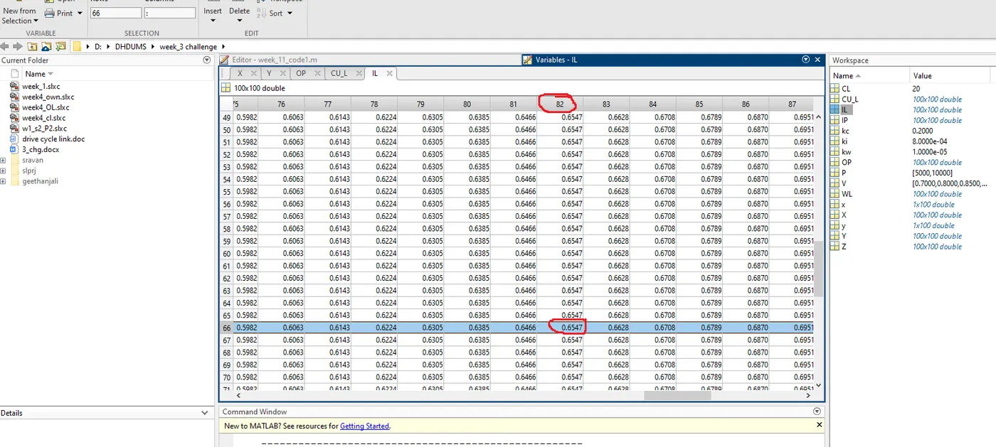
= 0.0008*818.364
= 0.6546.
The corresponding workspace variable is as shown in the below figure.
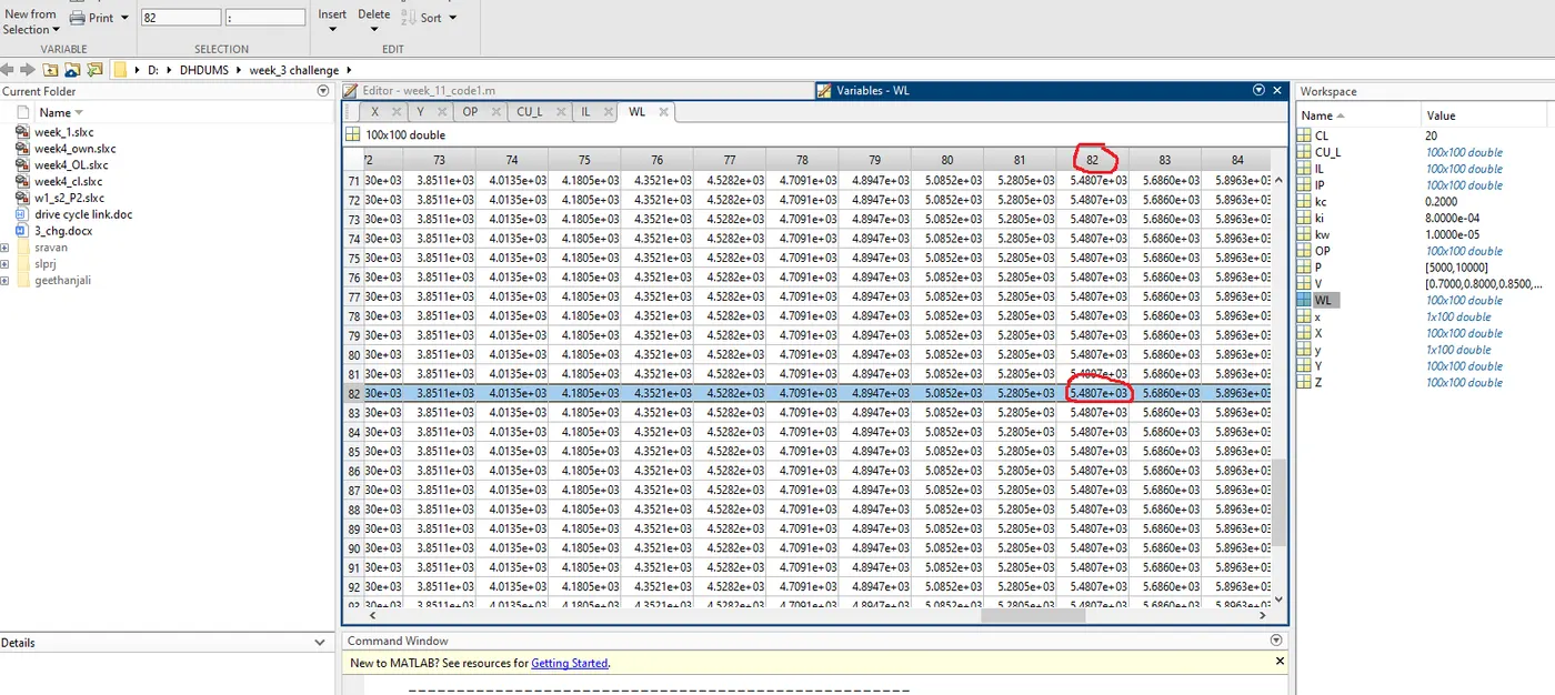
Windage loss= x.^3*kw
=818.364^3*0.00001
=5.48*10^3.
The corresponding workspace variable is as shown in the below figure.
Input power= Output power+cu_l+w_l+I_l+cl
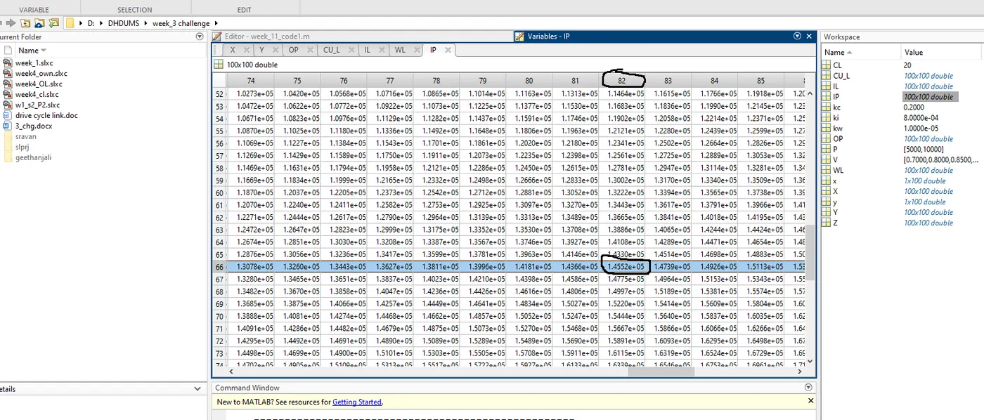
= (1.346*10^5)+(5.411*10^3)+(5.48*10^3)+0.6546+20
Input power = 1.455*10^5.
The corresponding workspace variable is as shown in the below figure.
Z= op/ip
=1.346*10^5/1.455*10^5
Z=0.925 or 92.5%
This efficiency(Level) is already represented in the contour plot as shown above.
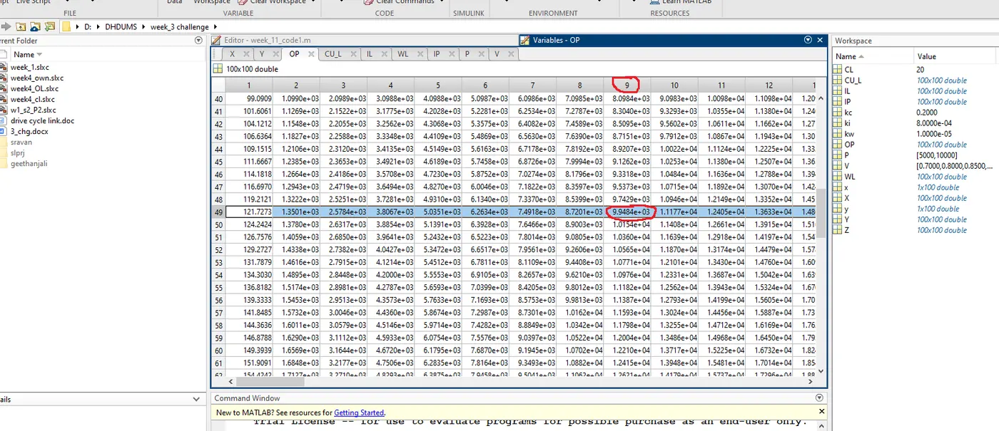
The output power for the 10kw curve is as shown in figure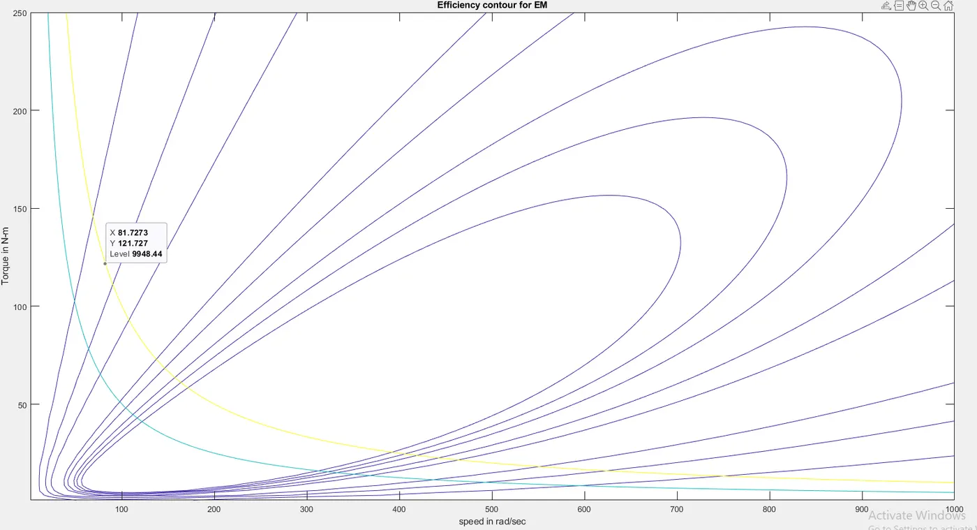
Output power =81.7273*121.72
Output power =9.947*10^3.
The corresponding workspace variable is as shown in the figure. In the above graph level nothing but output power.
Conclusion: Here i have taken two plots one is without efficiency vector and another one is with an efficiency vector. For the two cases mathematical validation has been done and verified with workspace results.