Project
Aim: To develop a technical content for ATV(All terrain vehicle) using MATLAB Simulink data.
Objectives: Explain the model properties ,carry out simulation of the vehicle and comment on the results.
ATV(All terrain vehicle):
An all-terrain vehicle (ATV) is defined as a motorized off-highway vehicle designed to travel on four low-pressure or non-pneumatic tires, having a seat designed to be straddled by the operator and handlebars for steering control. ATVs are subdivided into two types as designated by the manufacturer. Type I ATVs are intended by the manufacturer for use by a single operator and no passenger. Type II ATVs are intended by the manufacturer for use by an operator and a passenger, and are equipped with a designated seating position behind the operator. Similarly, riders must also consider the various ATV sizes.ATVs are not “one size fits all.” The ATV industry recommends all riders operate an ATV intended for their age. Youth model ATVs are designed for smaller hands and feet, and travel at slower speeds appropriate for their age.Every ATV made by our Members comes with a warning label with the manufacturers’ minimum age recommendation.
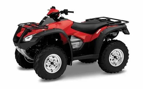
Fig.1 ALL TERRIAN VEHICLE(ATV)
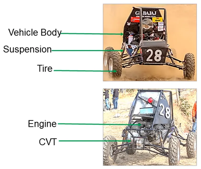
Fig .2 Parts of BAJA ATV
Simulink model of BAJA ATV using CVT:
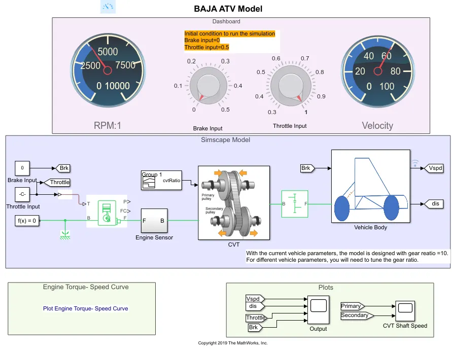
Fig.3 Simulink Model of BAJA ATV Using CVT.
Blocks Used:
1. Signal Builder.
2. Generic Engine.
3. Engine sensor.
4. CVT (Continuous Variable transmission).
5. Simple Gear.
6. Vehicle body.
7. Scope.
8. Goto and From.
9. Custom Gauge.
10.knob.
11. solver configaration.
12. Constant Blocks.
13. Mechanical rotational Reference Block.
CVT(Continuous Variable Transmission):A continuously variable transmission (CVT) is an automatic transmission that can change seamlessly through a continuous range of gear ratios. This contrasts with other transmissions that provide a limited number of gear ratios in fixed steps. The flexibility of a CVT with suitable control may allow the engine to operate at a constant RPM while the vehicle moves at varying speeds.
A CVT is similar to an automatic in that it doesn't use any input from the driver, but that is where the similarities end. A CVT doesn't have any gears. Instead, it has two pulleys. One pulley connects to the engine, and the other connects to the wheels. A flexible belt connects the two pulleys.The width of the pulleys changes depending on how much power the vehicle needs. When one pulley gets larger, the other one gets smaller. Since neither the pulleys or the belt are fixed, they can provide an infinite number of gear ratios, unlike the automatic, which has a set number of gears.Not all CVTs are created the same. The most common type is the pulley-based, but some other types include the Toroidal CVT, which uses rotating discs along with power rollers to produce the same result as the pulleys. The hydrostatic CVT uses pumps to control fluid flow, which then produces a rotational motion.
Advantages of CVT:
Depending on the vehicle and the driver, a CVT can provide a smoother driving experience when comparing it to a traditional automatic.
According to Carfax, one of the most significant advantages to having a CVT is that they are often more fuel-efficient than a regular automatic. This is part of the reason that they are becoming a more popular choice for automakers in many vehicles.
Disadvantages of CVT:
While the lack of upshifting and downshifting is considered an advantage of the CVT, some drivers miss the sensation of the vehicle moving through the shift points. If you prefer a sportier driving experience, then the lack of fixed gears makes the ride less engaging.Another complaint that drivers tend to make about a CVT is the loud droning sound that occurs during acceleration. This happens because the CVT forces the engine to continuously run a constantly high rpm as it gets up to speed.
As Car Engineer explains, the general public has been less accepting of the CVT due to the difference in noise perception from mechanical or step automatic transmission.CVTs can be expensive to repair or replace when compared to a conventional automatic transmission.
Some of the common problems that owners run into include overheating, slipping, and sudden loss of acceleration. Shuddering is also a common problem.
Since CVTs depend on the belts to operate, if these suffer from excessive stretching or too much wear, the transmission can completely fail.
Connections:
The constant blocks names indicated as Brake input and Throttle input. The output of Throttle input is connected to simulink to ps converter and it is connected T port of Generic Engine. For solver configaration block a mechanical translational reference is connected.The solver configaration is connected to B terminal of Generic engine. The output port F is connected to Engine sensor of F port and B port of engine sensor is connected to CVT Block and also CVT Ratio is connected to the CVT Block. The Output of CVT Block is connected to B terminal of simple Gear block. The output F is connected to vehicle Body and Brake input is also connected to the vehicle body and the output of vehicle body is velocity and distance. The CVT primary and secondary RPM are connected to the CVT shaft speed SCOPE and Vspd, dis, Throttle and Brake is connected to Output Scope. In this mode the engine speed torque characterstics are also provided.
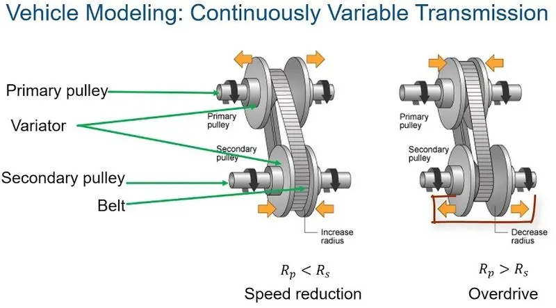
Fig 3. CVT with Primary and secondary Pulley.
CVT Block:
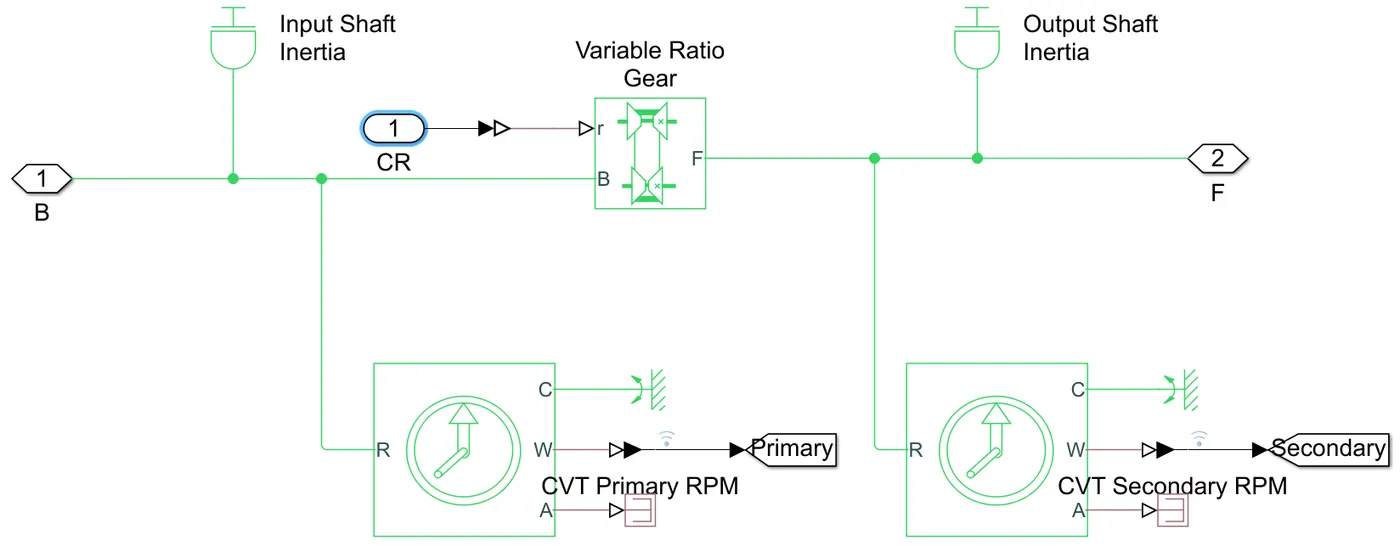
Fig 4 CVT Model.
In this CVT Block two shaft inertia blocks are used. one is Inpurt Shaft Inertia and other one is Output shaft inertia. Input shaft inertia is connected to B terminal of Engine sensor,R terminal of Rotational motion sensor and also to B terminal of Variable Ratio Gear.
The CVT Ratio CR is connected to the r terminal of Variable Ratio Transmission and F termina of Varibale Ratio Transmission is connected to Output shaft Inertia, R terminal of Rotational motion sensor and also to F terminal simple Gear.
The ideal motion sensor1 is connected to the CVT Primary RPM and ideal motion sensor2 is connected to the CVT secondary RPM.C terminal of ideal rotational sensor1 is connected to mechanical rotational reference. W terminal is connected to PS to simulink converter and this connected to Primary GOTO block.C terminal of ideal rotational sensor2 is connected to mechanical rotational reference. W terminal is connected to PS to simulink converter and this connected to Secondary GOTO block.
Vaiable Ratio Transimisson :Represents a variable ratio gearbox such as implemented by mechanical belt CVT, electric, or hydraulic transmissions. The physical signal input r defines the ratio of input to output angular shaft velocities.
Connections B (base) and F (follower) are mechanical rotational conserving ports. Specify the relation between base and follower rotation directions with the Output shaft rotates parameter.
The Variable Ratio Transmission block also represents a gearbox that dynamically transfers motion and torque between the two connected driveshaft axes, base and follower.Ignoring the dynamics of transmission compliance, the driveshafts are constrained to corotate with a variable gear ratio that you control. You can choose whether the follower axis rotates in the same or opposite direction as the base axis. If they rotate in the same direction, ωF and ωB have the same sign. If they rotate in opposite directions, ωF and ωB have opposite signs.Transmission compliance introduces internal time delay between the axis motions. Therefore, unlike a gear, a variable ratio transmission does not act as a kinematic constraint. You can also control torque loss caused by transmission and viscous losses.
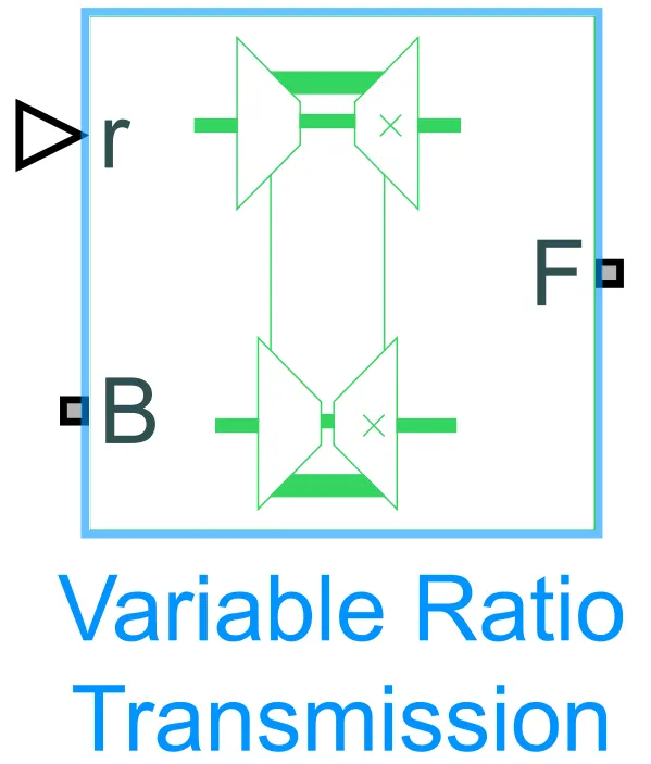
Fig.5 Variable Ratio Transmission.
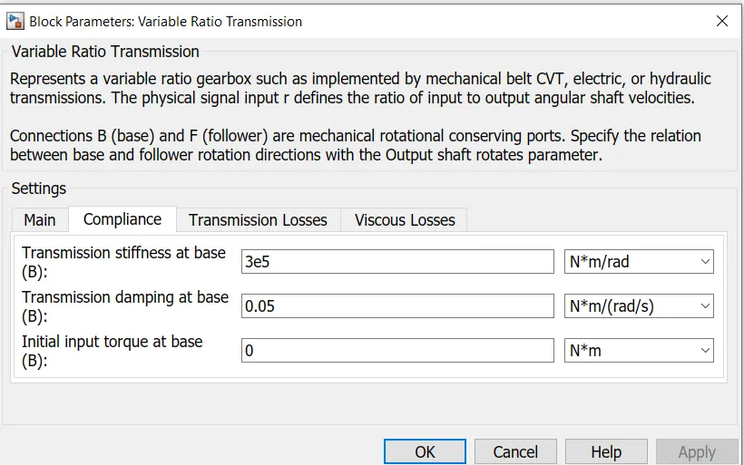
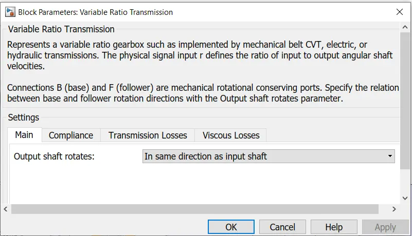
Fig .6 Compliance Values of Variable Ratio Transmission Fig .7 Output shaft position of Variable Ratio Transmission
Generic Engine:
The Generic Engine block represents a general internal combustion engine. Engine types include spark-ignition and diesel. Speed-power and speed-torque parameterizations are provided. A throttle physical signal input specifies the normalized engine torque. Optional dynamic parameters include crankshaft inertia and response time lag. A physical signal port outputs engine fuel consumption rate based on choice of fuel consumption model. Optional speed and redline controllers prevent engine stall and enable cruise control.
It also Represents a system-level model of spark-ignition and diesel engines suitable for use at initial stages of modeling when only the basic parameters are available. Optional idle speed and red line controllers are included.
The throttle input signal T lies between zero and one and specifies the torque demanded from the engine as a fraction of the maximum possible torque. If the engine speed falls below the Stall speed, the engine torque is blended to zero. If the engine speed exceeds the Maximum speed, the simulation stops and issues an error message.
Connections F and B are mechanical rotational conserving ports associated with the engine crankshaft and engine block, respectively. Connections P and FC are physical signal output ports through which engine power and fuel consumption rate are reported.
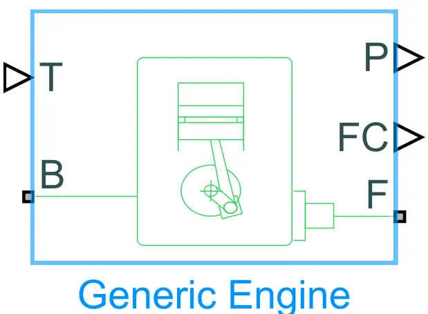
Fig 8. Generic Engine.
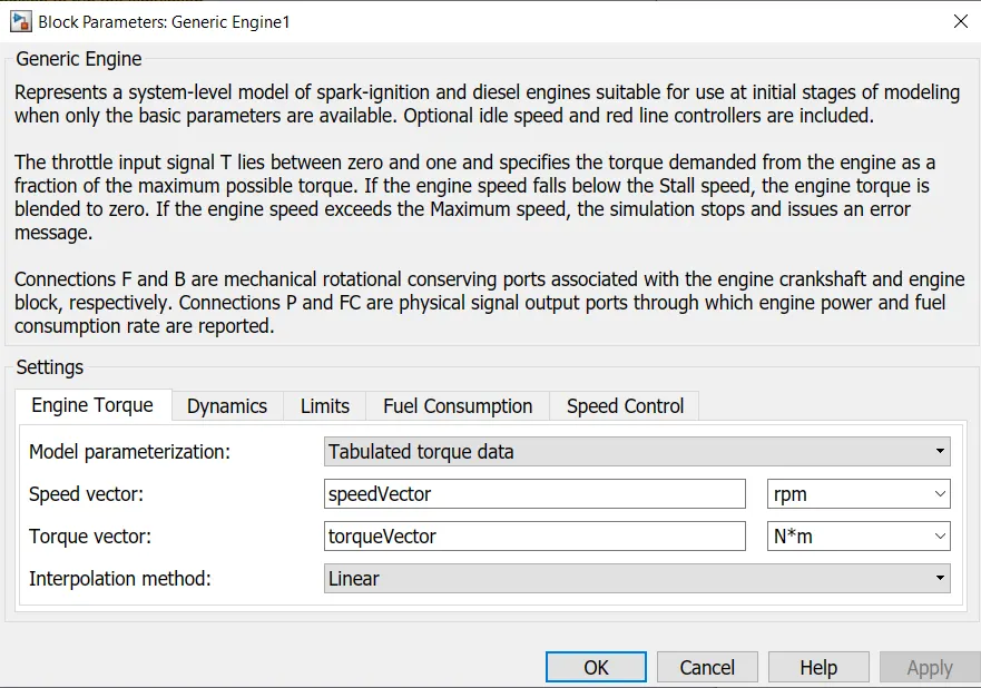
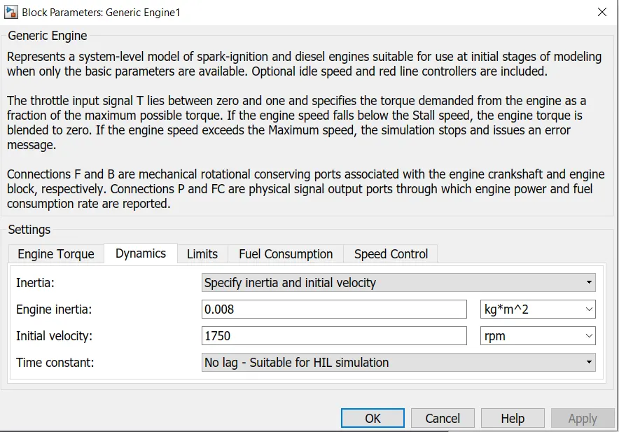
Fig 9. Generic Engine Torque parameters. Fig 10. Generic Engine Dynamics parameters.
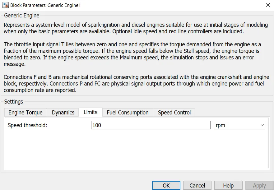
Fig 11. Generic Engine Limits.
Simple Gear:
The Simple Gear block represents a gearbox that constrains the connected driveline axes of the base gear, B, and the follower gear, F, to corotate with a fixed ratio that you specify. You choose whether the follower axis rotates in the same or opposite direction as the base axis. If they rotate in the same direction, the angular velocity of the follower, ωF, and the angular velocity of the base, ωB, have the same sign. If they rotate in opposite directions, ωF and ωB have opposite signs.
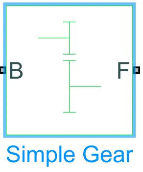
Fig. 12 Simple Gear.
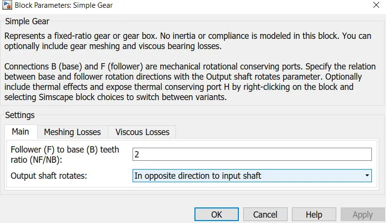
Fig. 13 Simple Gear main parameters
Ideal Rotational Motion Sensor:
The Ideal Rotational Motion Sensor block represents an ideal mechanical rotational motion sensor, that is, a device that converts an across variable measured between two mechanical rotational nodes into a control signal proportional to angular velocity or angle. You can specify the initial angular position (offset) as a block parameter.The sensor is ideal since it does not account for inertia, friction, delays, energy consumption, and so on.
Connections R and C are mechanical rotational conserving ports that connect the block to the nodes whose motion is being monitored. Connections W and A are physical signal output ports for velocity and angular displacement, respectively.
The block positive direction is from port R to port C. This means that the velocity is measured as ω = ωR – ωC, where ωR, ωC are the absolute angular velocities at ports R and C, respectively.
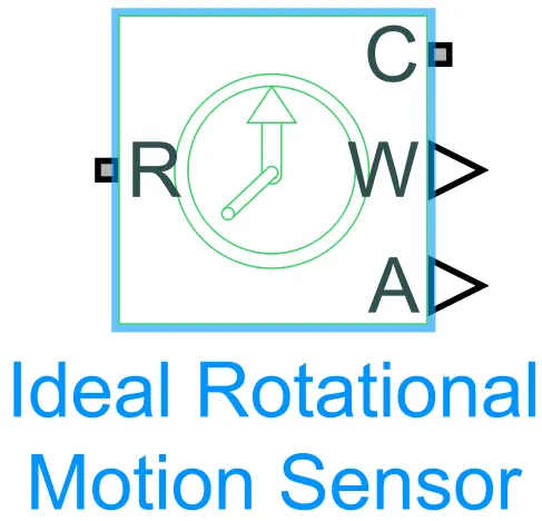
Fig.14 Ideal Rotational Motion Sensor.
Inertia:
The block represents an ideal mechanical rotational inertia.The block has one mechanical rotational conserving port. The block positive direction is from its port to the reference point. This means that the inertia torque is positive if the inertia is accelerated in the positive direction
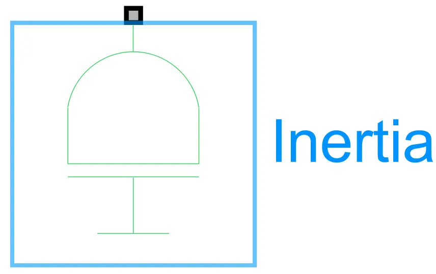
Fig.15 Inertia.
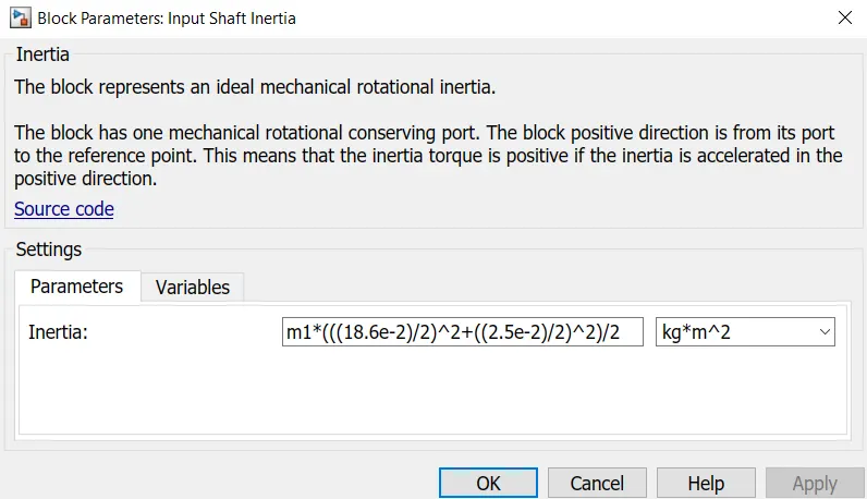
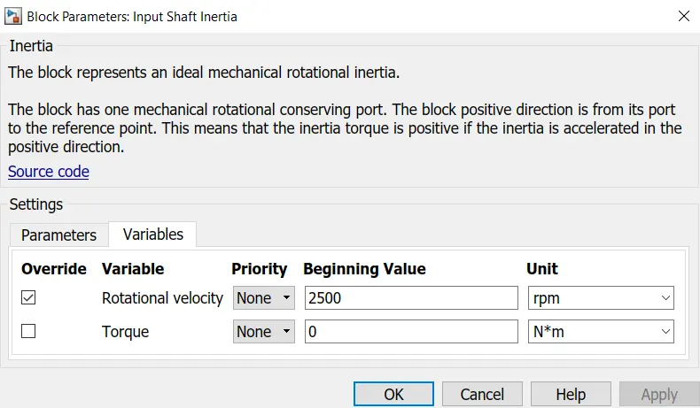
Fig.16 parameters of Inertia. Fig.17 Variables of Inertia.
Subsystem of Vehicle Block:
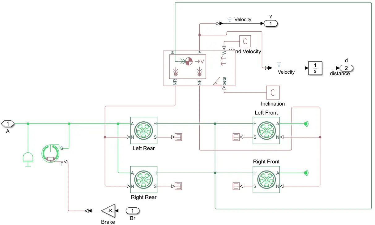
Fig.18 Subsystem of Vehicle Block.
F terminal of simple gear is connected to Inertia and double shoe brake port S and also to A port of Tire (Left Rear).Also NR ports of vehicle body is connected to N ports of Left and Right Rear and NF ports of vehicle body is connected to N ports of Left and Right Front. Wind Velocity and Inclination to W and beta of Vehicle Body. H port of vehicle body is connected to all tiers of H Blocks.
Vehicle Body:
The Vehicle Body block represents a two-axle vehicle body in longitudinal motion. The vehicle can have the same or a different number of wheels on each axle. For example, two wheels on the front axle and one wheel on the rear axle. The vehicle wheels are assumed identical in size. The vehicle can also have a center of gravity (CG) that is at or below the plane of travel.
The block accounts for body mass, aerodynamic drag, road incline, and weight distribution between axles due to acceleration and road profile. Optionally include pitch and suspension dynamics. The vehicle does not move vertically relative to the ground.
The block has an option to include an externally-defined mass and an externally-defined inertia. The mass, inertia, and center of gravity of the vehicle body can vary over the course of simulation in response to system changes.
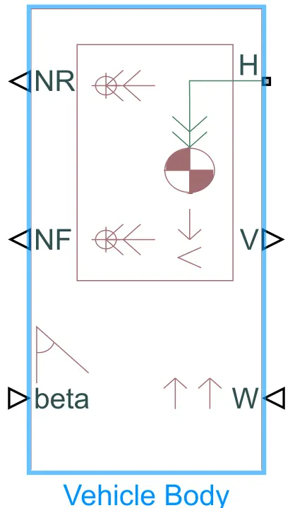
Fig.19 Vehicle Body.
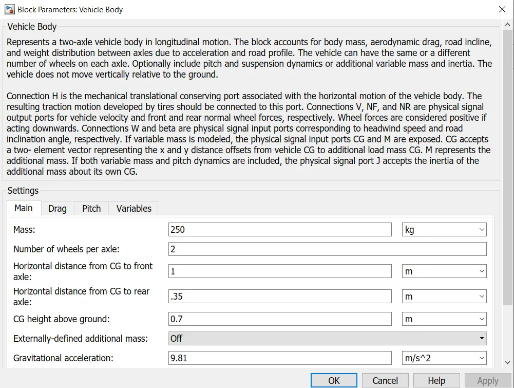
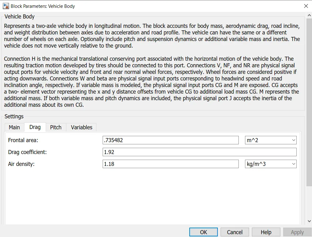
Fig.20 Main parameters of Vechicel Body. Fig.21 Main parameters of Vechicel Body.
Custom Gauge:
The Custom Gauge block displays the value of the connected signal on a gauge face that you can customize to look like a gauge in a real system. For example, you could create an engine rpm gauge or fuel indicator for an automotive model.The Custom Gauge block provides an indication of the instantaneous value of the connected signal throughout simulation. You can modify the range and tick values on the Custom Gauge block to fit your data. Use the Custom Gauge block with other Dashboard blocks to build an interactive dashboard of controls and indicators for your model.
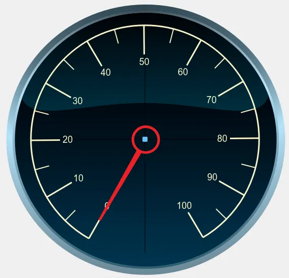
Fig.22 Custom Gauge.
In this model speed values considerd as O and 15,000Rpm for Rpm1 block shown in fig.3 and another block name is Velocity(km/hr) and the values considered are 0 and 100 shown in fig.3.
Knob:
The Knob block tunes the value of the connected block parameter to during simulation. For example, you can connect the Knob block to a Gain block in your model and adjust its value during simulation. You can modify the range of the Knob block's scale to fit your data. Use the Knob block with other Dashboard blocks to create an interactive dashboard to control your model.
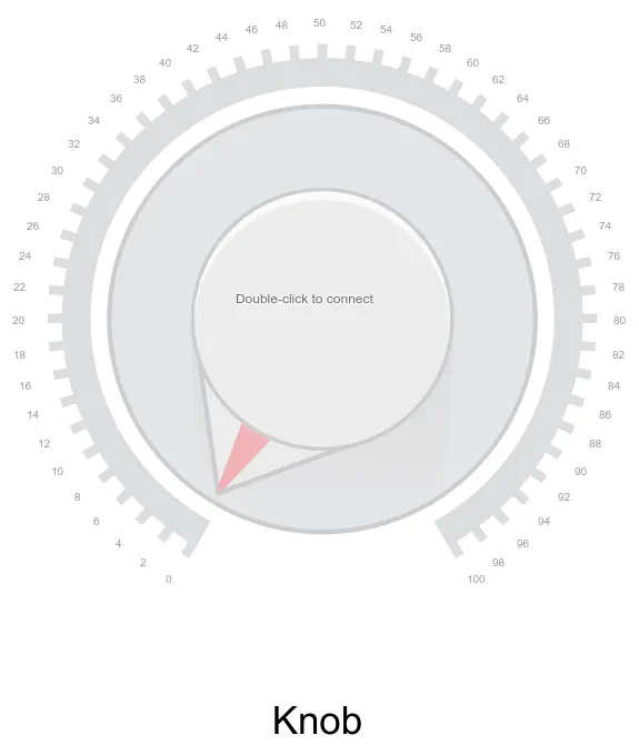
Fig. 23 Knob
In this model for Brake input the values are considered as 0 and 0.5 and for Throttel input the values are considered as 0 and 1 shown in fig.3.
Signal Builder For CVT:
The CVT Ratio is maintained 2.9 upto 6secs and linearly decreasing upto 35 secs and maintained a constant value of 1.3.
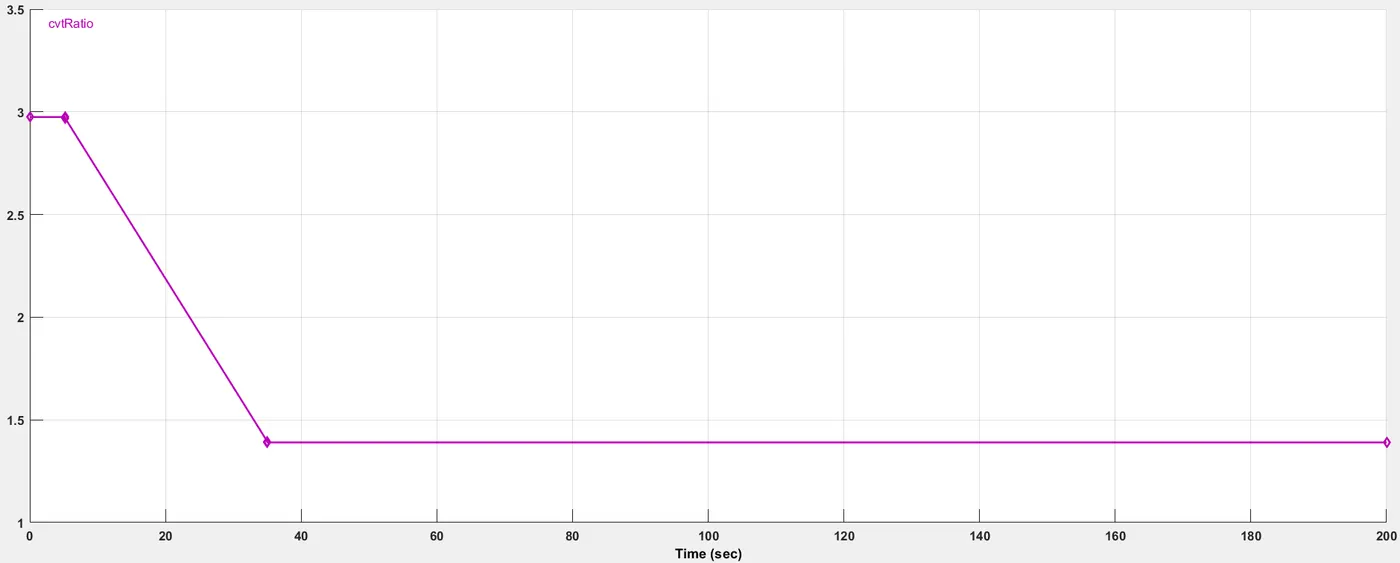
Fig. 24 Signal Builder for CVT
Casei: Brake is equal to 0 and Throttle is 0.5.
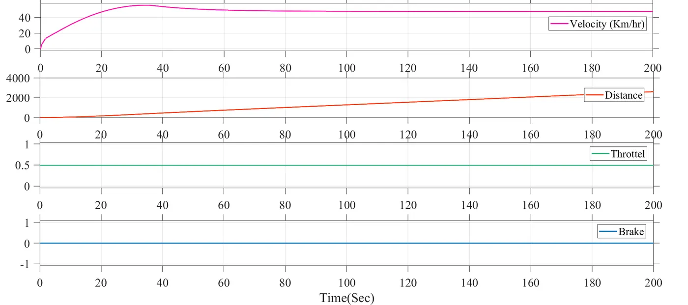
Fig .25 Output Waveforms.
From the above waveforms it is clear that at t=35sec maximum velocity is obtained and the value is 55.5Km/hr. Once it reaches the steady state velocity reaches to 47.6 Km/hr. Coming to the distance initially it is zero and it is increasing linearly and at the end of the simulation i.e at t=200sec the distance reachest ot 2550m. It is observed that throttle value is 0.5 and Brake value is 0 and the corresponding waveform is shown in fig.25.
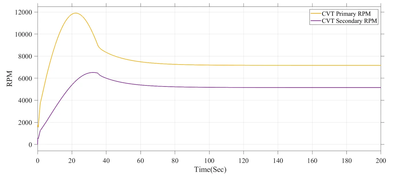
Fig .26 CVT Waveforms.
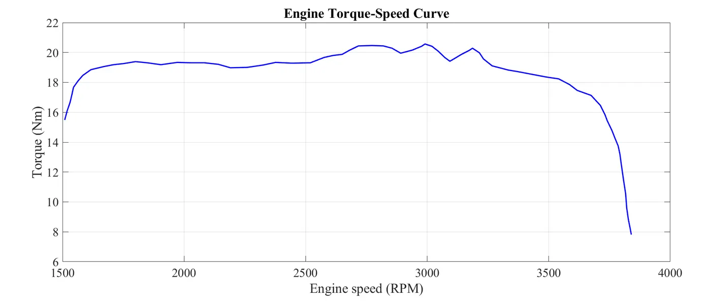
From the above waveforms it is clear that at t=20sec the primary RPM reached max value and it is nearly 12000 and secondary RPM reached max value at t=35sec. The primary RPM reaches steady state value of 7167RPM and secondary RPM reaches steady state value of 5155 RPM. The corresponding Engine Torque-speed Curve as shown in below figure.
Caseii: Brake value is varying and Throttle is 1.
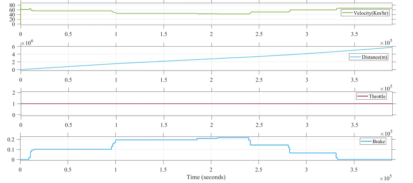
Fig.27 Output Waveforms
From the above waveforms it is observed that if the brake value is increases the velocity is reduces from (0.1*10^5)sec to (2.4*10^5)secs and the if the brake value is decreases then the velocity is increases from (2.4*10^5)sec onwards
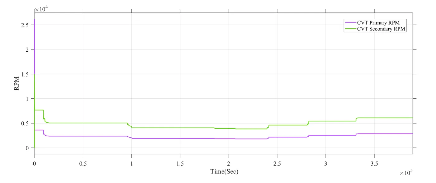
Fig .28 CVT Waveforms.
It is also observed that CVT Rpm of Primary and secondary waveforms are reduced upto (2.4*10^5) because brake value is increases and from (2.4*10^5) onwards the brake value is decreases therefore the CVT Primary and secondary RPMs are increases.
case iii: Brake value is varying and Throttle is value is varying.
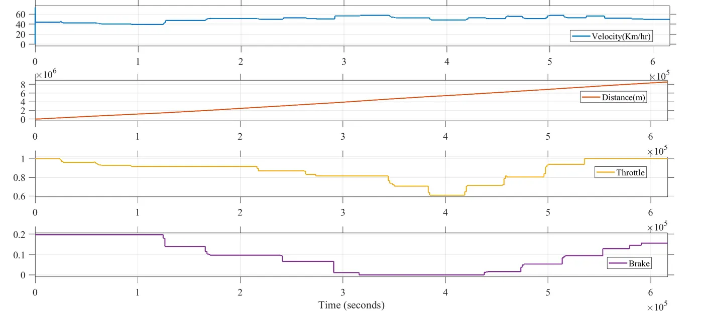
Fig.29 Output Waveforms
From the fig.29 it is observed that brake and throttle both are varying. The brake value is changed with wide range when compare to throttle value change. Intitally the throttle value is reduced then the velocity is reduces and later brake value is changed from 0.2 to 0.13 there the velocity starts increases. After t=(4*10^5)sec brake and throttle are increasing there fore speed increases slightly because increase in throttle value is greater than brake value. It is observed that distance increases linearly and reaches (8*10^5)m.
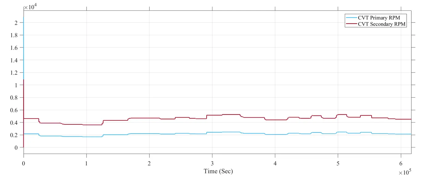
Fig .30 CVT Waveforms.
From Fig.30 it is observed that initially CVT RPM is reduces because change in throttle value is greater than Brake value. After (1*10^5)sec the speed is slightly increasing because the Decrease in brake value is more than throttle value. This will happen upt0 (4*10^5).After that CVT RPM is decreases and increases because of the change is throttle as well as brake value.
Case iv: Brake is 0.1 and throttle is varying.
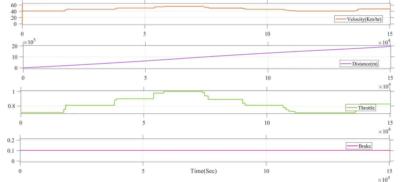
Fig.31 Output Waveforms
From the Fig.31 it is observed that brake value is fixed as 0.1 and the throttle value is changed. when the throttle value is increases then the speed increases and decreases when throttle value is decreases.
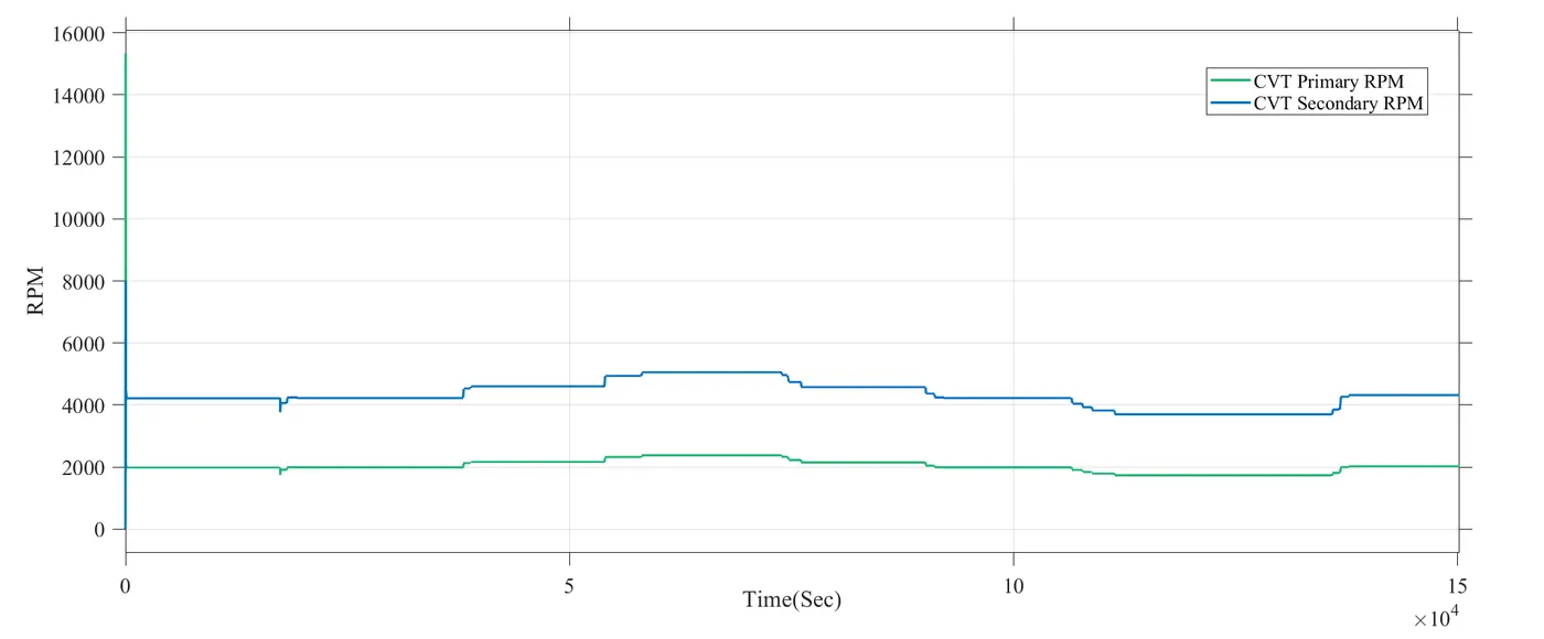
Fig .30 CVT Waveforms.
For CVT RPM also when the throttle value increases the CVT RPM increases and decreases when the throttle value is decreases.