Braking and Motor Efficiency Contour Plots

Q1. For a defined driving cycle, calculate the energy required for braking.

Ans :

The driving cycle chosen is : Arterial Segment of the Transit Coach Operating Duty Cycle

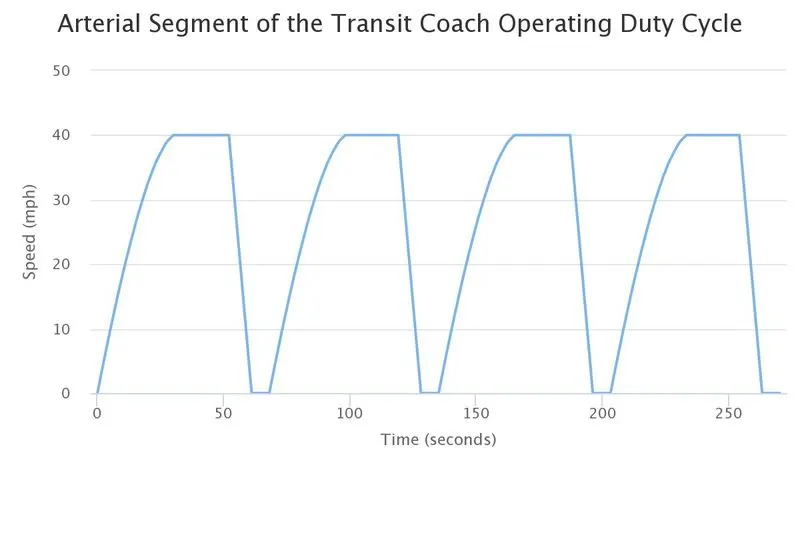
Mass taken is 800 Kg

Vehicle brakes from 40 mph to 0 mph in 9 sec. The calculations can be seen in the attached excel file.

Braking Power Needed = 14.21 kW

Total Time = 270 sec

Total braking energy = 0.1421 kWh

Q2.Why electric motor can’t develop braking torque at high speed similar to starting? How electric and mechanical brakes are coordinated?

Ans:

At start, we can apply the rated or maximum current with the maximum flux.

Torque = k*Flux*Current

where k is a constant

In the high speed region, the flux weakening is applied. Thus flux reduces in the airgap. Even with maximum current, the braking torque cannot be same as that of starting.

Thus braking torque at high speed < Starting torque

Electric and mechanical brakes need to be coordinated by the different brake control strategy:

1. Series Brake Control Strategy : In this, strategy, the regenerative braking is first applied and then the mechanical brakes are applied until vehicle comes to stop.

2. Parallel Brake Control Strategy : Here, both regenerative and mechanical brakes are applied at the same time.

3. Electric Drive Intelligent Brake : Initially regenerative braking is used and then both regenerative and mechanical brakes are used to get maximum energy efficiency and comfort.

Q3. Make a MATLAB program which plots contour of given motor speed, torque and efficiency values. Attach the code as a .m file attach a screenshot of all the plots.

Ans:

x = linspace(1,1000); %speed
y = linspace(1,250); %Torque

%Loss constants
kc = 0.2; % For copper loss
ki = 0.008; %For iron loss
kw = 0.00001; %For windage loss
c = 20; %constant loss

%mesh 
[X,Y] = meshgrid(x,y);
Outputpower = (X.*Y); %power = torque * speed
B = (Y.^2)*kc; %copper loss
C = X*ki; %Iron Loss
D = (X.^3)*kw; %Windage loss
Inputpower = Outputpower + B + C + D + c;
Z = Outputpower./Inputpower;

%Efficiency at which a contour will be plotted
V = [0.6,0.7,0.75,0.8,0.85,0.9,0.91,0.92,0.93,0.94,0.95];
box off
grid off
contour(X,Y,Z,V)
xlabel('Speed/rad.s^-^1'),ylabel('Torque/N.m');

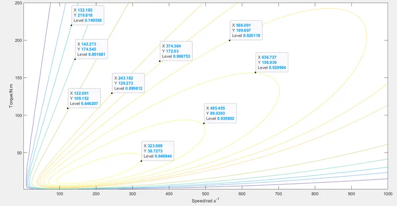
Here we can see the efficiency contour plots for the following range :

Torque Range : 0 to 250 Nm

Speed Range : 0 to 1000 rad/s

Efficiency Range : 60%, 70%, 75%, 80%, 85%, 90%, 91%, 92%, 93%, 94% and 95%