Design of an Electric Vehicle with MATLAB and ADVISOR Tool

Final Project: Design of an Electric Vehicle

For the project, a cargo vehicle is simulated, which is able to carry a load of 500 Kg. ADVISOR tool is used to estimate the motor rating. FTP driving cycle is used for both the ADVISOR model and the MATLAB Simscape model. It is verified that the simulated EV model is able to mee the FTP driving cycle standards.

Vehicle Parameters :

Drive train : Pure Electric Vehicle

Vehicle Type : Small Cargo Vehicle

Battery Pack : Li-ion Battery Pack (25 Modules)

Nominal Voltage : 308 V

Motor : 75 kW (Rated Power) DC Motor

Net Vehicle Mass : 1784 Kg

Payload : 500 Kg

Width : 1.765 m

Height : 1.595 m

EV Motor Power Calculations (Low Tyre Pressure)	Default EV
Rolling Resistance
Curb Weight (Kg)	1784
Payload(Kg)	500			Default EV
Coefficient of Rolling Resistance (urr)	0.0222
Rolling Resistance Force (N)	496.90704			Tyre 215/50R17
			Dia	646.8	mm
Air Drag Calculation			Radius	0.3234	m
Air Density (Kg/m3)	1.25
Width (m)	1.765		Total Traction Force	4523.50925354167	N
Height (m)	1.595
Frontal Area (m2)	2.815175		Gear	7	(1:7 Gear Ratio)
Drag Coefficient	0.2
Speed(kmph)	90		Wheel Torque (Nm)	1462.90289259538	(Maximum)
Air Drag(N)	219.935546875
			Motor Torque (Nm)	208.986127513625	(Maximum)
Total Power at given speed (kW) Air Drag + Rolling Resistance	17.921064671875	kW
			Speed of axel	77.3036487322202	rad/s
Hill Climbing
Angle (Degree)	0		Speed of shaft	541.125541125541	rad/s
Speed during hill climbing (kmph)	25
Force(N)	0		Power (Rated)	113.087731338542	kW
Hill Climbing Power (kW)	0	kW
Acceleration Calculation
Final Speed (0 to x kmph)	90
Acceleration Time (sec)	15
Acceleration (m/s2)	1.66666666666667
Acceleration (N)	3806.66666666667
Acceleration Power(kW)

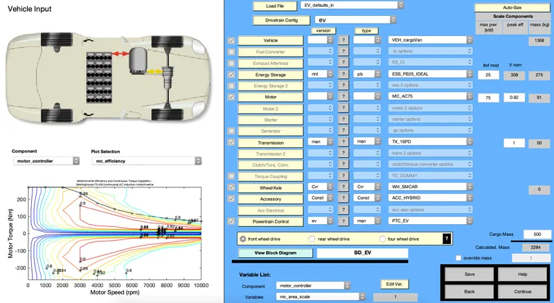
Fig 1: Vehicle input design with ADVISOR tool

We need to test the motor on the FTP driving cycle. The ADVISOR tool is used to verify that the motor and battery rating is suitable for the driving cycle.

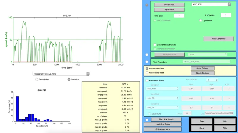
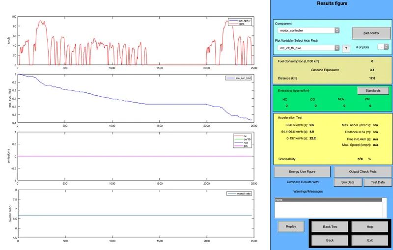
Fig 2: Vehicle design and analysis for FTP cycle using ADVISOR tool

The MATLAB model has five components :

1. Vehicle Body : It includes the vehicle body, tires and gear

2. Electrical System: It includes the power converter and dc motor

3. Battery : It includes calculation of State of Charge and battery model

4. Driver: It includes the control of throttle based on driving cycle

5. The drive cycle.

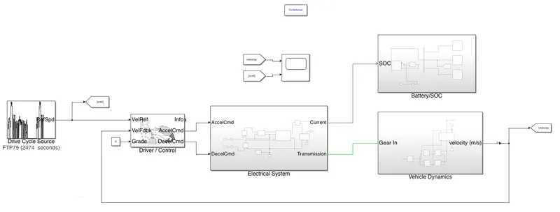
Fig 3 : System Level Design

1. Vehicle Dynamics

It constitutes of the vehicle body, load, gear and the tire. We will look into each in detail.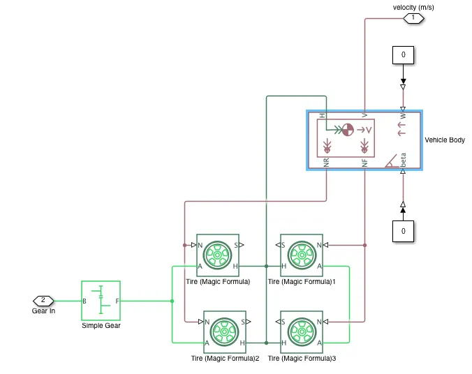

Fig 4 : Vehicle Dynamics

The vehicle body has the total mass of 2284 as calculated from the ADVISOR tool. There are two axels and two wheels on each axel. The frontal area of the vehicle is 2.815 m^2 for the calculation of drag force. H is the connection or horizontal movement of vehicle. W is the road incline angle, which we have taken as 0. The outputs are V or the velocity, in m/s. NF and NR are the front wheel and rear wheel force.

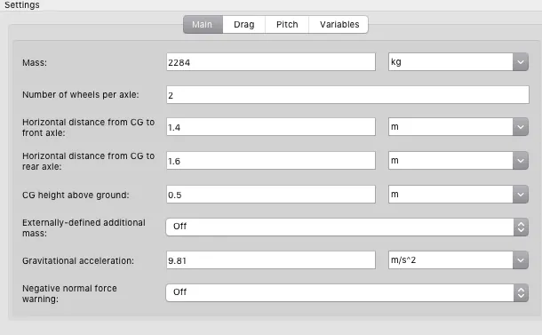
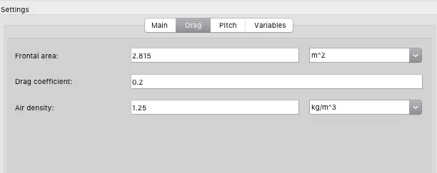
Fig 5 : Vehicle Body Parameters

The tires are modelled based on the longitudnal traction force. The peak traction force calculated is 4500 N which has been used as a parameter. The nominal force is taken as 4500 N. The Tire (Magic Formula) block is used here. Output here is the slip. The radius of wheels is taken as 0.3234 m which is same as for 215/50R17 model.

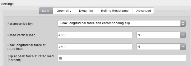
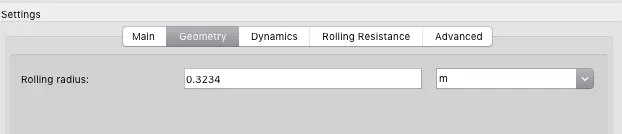
Fig 6 : Tire Paramters

The transmission gear box in electric vehicle has a single gear ratio. The gear ratio chosen is 7. The output and input shaft rotate in the same direction.

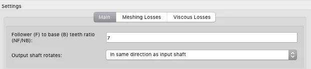
Fig 7 : Gear Ratio

2. Electrical System

The electrical system consistes of the power converter and DC motor. The throttle output is controlled by the driver. This output is the control signal for generating PWM signals for power converter. The power converter used here is 4-quadrant H bridge. This converter can work in all four quadrants and can be used for regenerative braking as well. Here a PMDC motor is used. The field is provided by permanent magnets. Here, solver configuration is set to use the Backward Euler solver, which increases the simulation speed significantly. The number of iterations are also high to get greater accuracy.

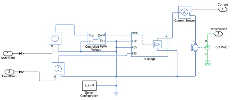
Fig 7 : Electrical System

The DC motor is using permanent magnets for in the stator. The rated output of the motor is the same as calculated from the ADVISOR tool i.e. 75 kW. The rated DC supply is 38 V. The block assumes that no electromagnetic energy is lost, and hence the back-emf and torque constants have the same numerical value when in SI units. When a positive current flows from the electrical + to - ports, a positive torque acts from the mechanical C to R ports. Motor torque direction can be changed by altering the sign of the back-emf or torque constants.

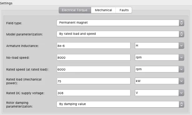
Fig 8 : DC Motor

The H Bridge is 4 quadrant DC-DC converter. It has four switches and can work in all four quadrants, i.e. Forward Motoring, Forward Braking, Reverse Motoring and Reverse Braking. In the drive cycle, only forward motoring and forward braking mode is used. The battery gets depleted in the forward motoring mode as the DC machine absorbs power and acts as a motor. In the forward braking mode, the SOC of battery increase, as the battery gets charged. This is possible since the DC machine acts as a generator in the 2nd quadrant / regenerative braking mode. An internal power source of 308 V is provided. With the duty ratio of 100% the nominal voltage of 308 V is obtained at the output of the H bridge.

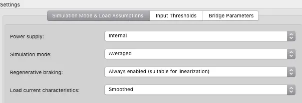
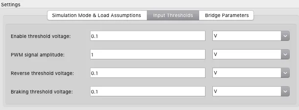
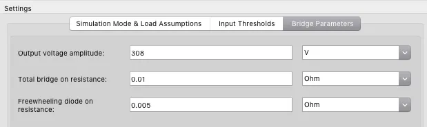
Fig 9: H Bridge Parameters

The gate signals are generated using Pulse Width Modulation technique. The carrier signal has the frequency of 5000 Hz. Acceleration command and Deceleration command vary from 0 to 100%. For a 0% signal, the controlled voltage source has a value of 0 V and for 100% throttle , the output voltage is 1. This throttle signal is the control signal for generating PWM signals. Fig 10 shows the 4-quadrant chopper circuit. Here the acceleration command controls the switching of S1 and S4. The deceleration command controls the switching of S2 and S3. The parameters for generating PWM signals can be seen in Fig 11.

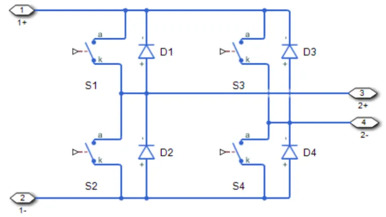
Fig 10 : 4-Quadrant Chopper

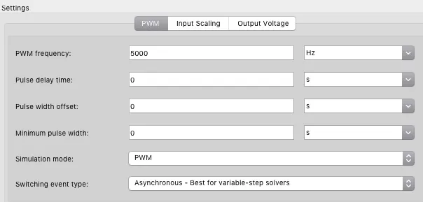
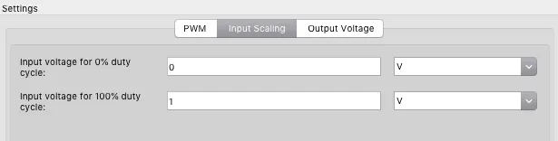
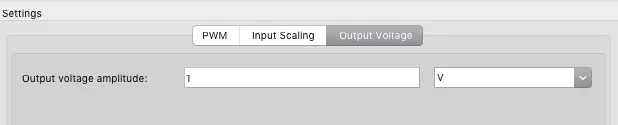
Fig 11 : PWM Controller Parameters

3. Battery / SOC

Here a rechargeable Li-ion battery pack is used. The battery SOC is calculated using the current flow through the battery. This is represented by a current source. The nominal voltage of the Li-ion battery as calculated from the ADVISOR tool is 308 V at 90% SOC. The rated capacity of the battery is 100 Ah. The battery parameters can be seen in Fig 13 and the discharge characteristic curves can be seen in Fig 14.

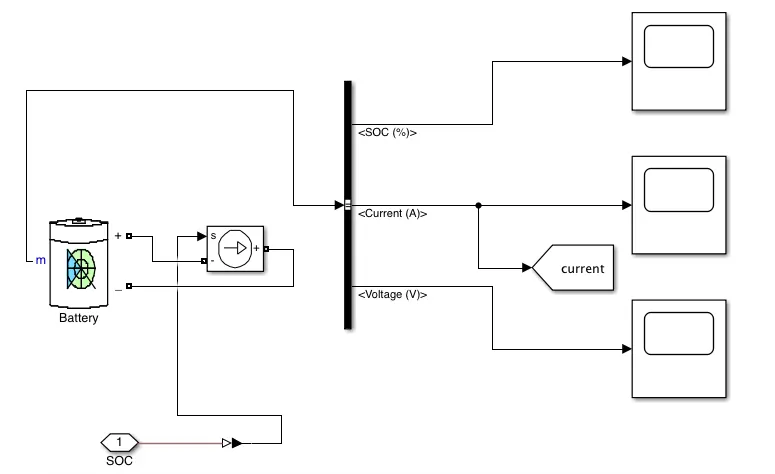
Fig 12: Battery System

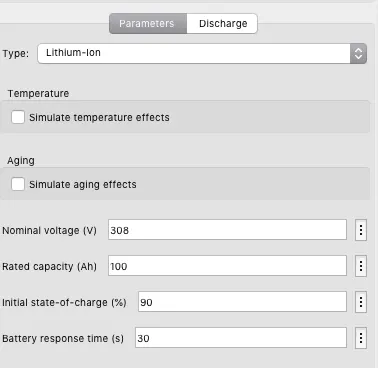
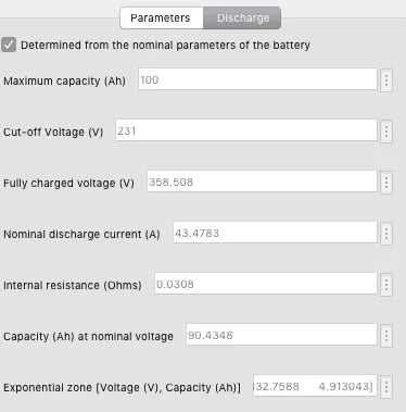
Fig 13 : Battery Parameters

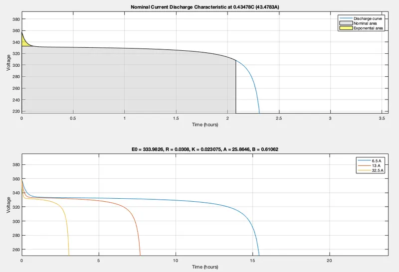
Fig 14 : Battery Discharge Curve

4. Driver :

The driver presses down on the throttle or applies brakes depending on the desired Driving Cycle and the incline/decline of the road or road conditions. This effect has been modelled using the Longitudnal Driver block. THis block generates the normalised acceleration and braking commands that vary between 0 and 1.

A predictive control is used here. Effective vehicle traction force and the rolling resistance force are the input parameters that are calculated through the excel sheet attached.

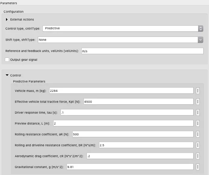
Fig 15: Longitudinal Driver Parameter

6. Drive Cycle :

The FTP drive cycle is used for simulation. This cycle runs for 2474 sec and covers 17.77 Km. The maximum speed is 91.25 Km/h and average speed is 25.82 Km/h. There are 22 stops in the cycle. The parameters can be seen in Fig 16 and the drive cycle (speed in m/s) can be seen in Fig 17.

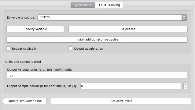
Fig 16: Drive Cycle Parameter

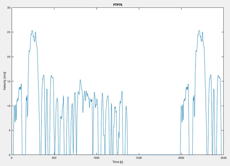
Fig 17 : FTP75 Drive Cycle (Speed in m/s)

RESULTS

The actual speed and the reference speed from drive cycle are compared here. The results can be seen in Fig 18. The controller is working for most of the driving cycle. The controller needs to be further tuned for better speed control. Moreover, physical brakes have not been implemented in the model, do, the vehicle takes more time to decelerate. It is clear that 100% energy cannot be recovered through regenerative braking. The State of Charge % can be seen in Fig 19. THe SOC is 90 % at the start of the driving cycle. It is 86.4% at the end of the cycle. The SOC increases during deceleration due to regenerative braking.

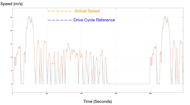
Fig 18 : Reference speed v/s actual speed

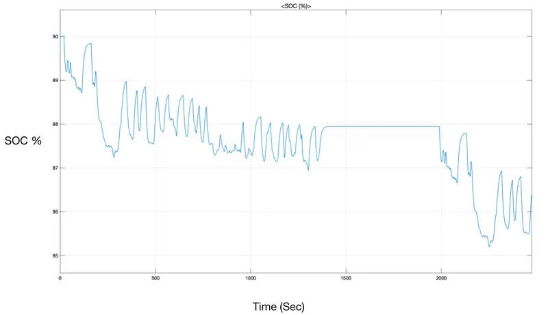
Fig 19 : Battery SOC

Conclusion

The Simulink Model of an electrical vehicle is presented here. Powertrain blockset is used here, which simulates the real world electrical and mechanical systems. This is however, a very simple model. The controller and solver have to be tuned properly to get correct results. First, Wide Open Throttle (WOT) test was conducted for a sanity check on the parameters. This is done using the motor rating obtained with ADVISOR tool and simple parameters obtained using excel sheet. Then the FTP drive cycle is evaluated.

It is observed that acceleration is faster than the deceleration. This is true in real world as well since the discharge rate of battery is generally more than the charging rate. Mechanical brakes and current limiter circuit are needed better braking action and faster response. Controller also needs to be tuned to get accurate and fast results. Speed of simulation depends on the solver configuration., thus it should be chosen carefully.

The model is able to complete the drive cycle with only 4% reduction in SOC at the end of drive cycle. The high amount of regenerative energy is fed back to battery as others losses like heat, noise and vibration are not taken in the simulation. However, this model proves that the given motor, power converter and battery pack can be used for this electric vehicle application.