Braking Energy calculation for FTP75 drive cycle using Simulink, brake system control strategy and Efficiency map of SPM AC machine using MATLAB

1. For a defined driving cycle, calculate the energy required for braking.

Solution 1:

One of the most significant feature of the EV is its ability to recover significant amounts of Braking Energy .

Braking perfromance of a vehicle is a very important consideration for safety. which requires 2 things:

1. ability to reduce speed of the vehicle quickly as demanded
2. maintiaining vehicle direction while brakes are being applied

which is done by :

1. providing sufficient amount of Braking torque
2. Proper distribution of brake force among the wheels

usually the motor cannot provide the high Braking torque on its own this is why a Hybrid braking system is used which is a combination of both mechanical/conventional and Electric/Regenerattive braking.

Power at any instant is :

`=>P = V/1000 (Mgf_r + 1/2rho_aC_dAV^2 + Mdelta(dV)/dt)` kW

where M is mass of the vehicle,`f_r` is coefficient of friction, `rho` is air density, A is frontal Area of the vehicle, V is velocity of the vehicle, `delta` is rotational inertia factor to include the effect of roatating parts and (dV)/dt is the rate of cvhange of speed.

for P>0 : then the Traction wheels are recieving power from the energy source and the vehicle moves forward

for P<0 : then here braking is applied, and the kinetic energy of the vehicle is dissipated by the brake system.

integration of the Power equation will give use the energy in each case, Traction or Braking.

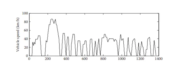
Fig: FTP75 Drive cycle shown for 1400 s

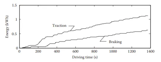
Fig: Traction and Braking energy corresponding ot the FTP75 drive cycle above

So we see a the braking energy seems to be a significant percentage of the Traction energy. So recovering this amount of ebergy will increase the efficiency of our Vehicle a lot. And this increases in case of Drive cycles that have frequenct start and stops. Example in New York city it can reach of upto 80% of the total Traction energy! and typical urban driving it is aorund 34%

there are many drive cycles such as EPA FTP75, LA92, US06, ECE-15,New York City, etc

we will be using the Urban FTP75 Drive cycle (1400 sec driving time)

looking at the drive cycle:

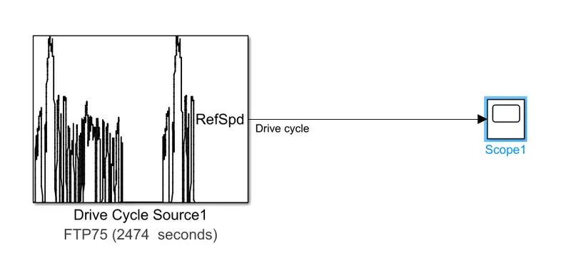
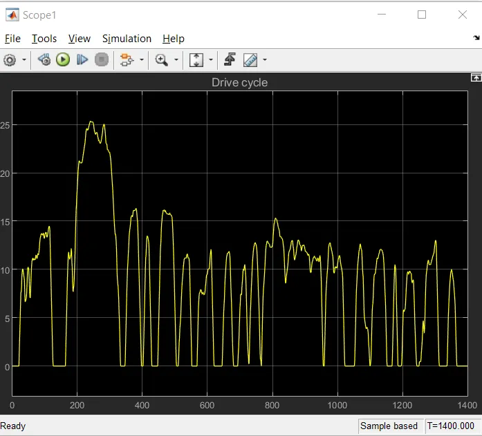
Fig: Drive cycle used visualized - FTP75 for 1400 sec

we will have to use our formula to compute the Power:

`=>P = V/1000 (Mgf_r + 1/2rho_aC_dAV^2 + Mdelta(dV)/dt)` kW

but also segment and divide the points according to acceleration and deceleration for Traction Energy and Braking Energy respectively

this is done by checking the sign of the derevative. if `(dV)/dt>0` then it is accelearting and the Traction force is being applied and if the `(dV)/dt<0` it is decelerating and the Braking force is applied.

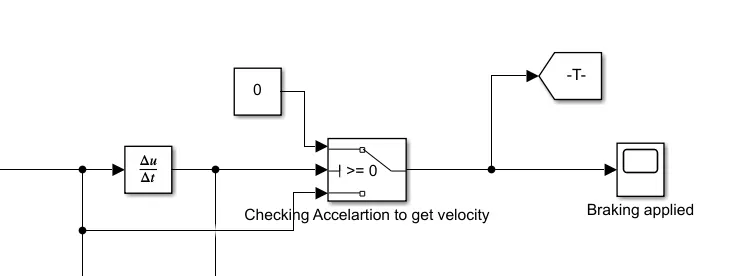
Fig: checking sign of the derevative to decide the points of the drive cycle that will be under Braking operation

this is implemented as a subsystem that takes input of the Drive cycle and creates the Velocity and Acceleration/Deceleration vector according to the derevative sign.

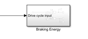
Fig: takes input of the Drive cycle and creates the vector of Braking velocity and the Braking deceleration

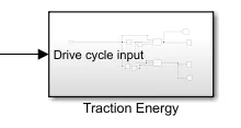
Fig: takes input of the Drive cycle and creates the vector of Traction velocity and the Acceleration

outputs of this we see below (2 from both blocks, acceleartion values and the corresponding velocity)

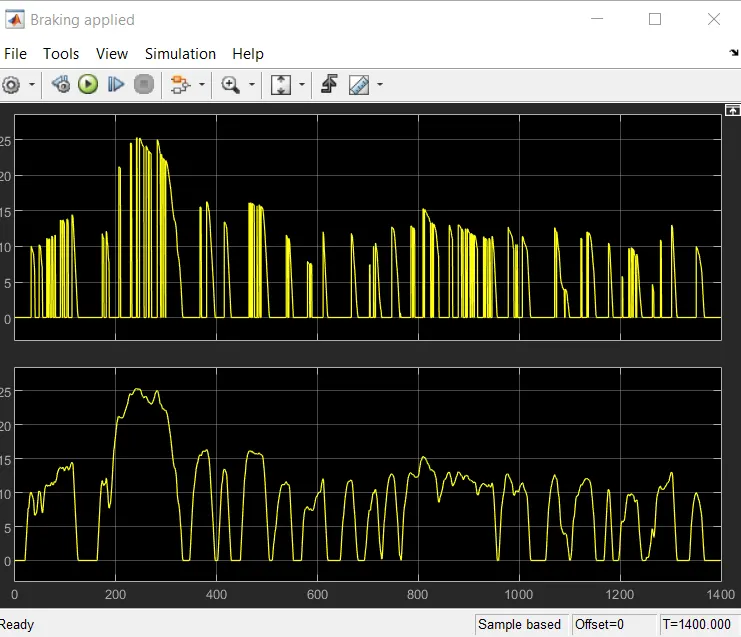
Fig: Points where Braking is applied(top) with respect to the Drive cycle(below)

similatly we can also get the points where traction is applied

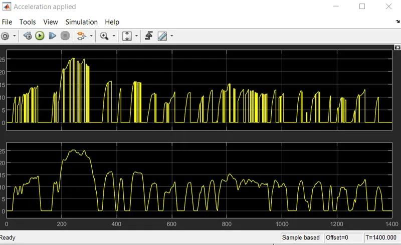
Fig: Points where Traction is applied(top) with respect to the Drive cycle(below)

we can also get the `(dv)/dt` in both the cases for our power calculation

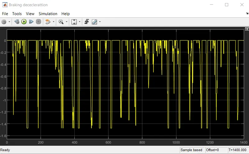
Fig: Deceleration value in the Drive cycle points notice `(dV)/dt<0`

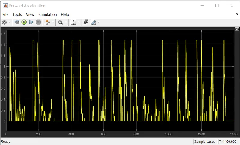
Fig: Deceleration value in the Drive cycle points notice `(dV)/dt>0`

Applying the Power formula for both cases . Traction and Braking :

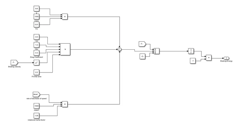
Fig: Model implmented to apply the power formula for Braking power. Velocity input is the part of the drive cycle when `(dV)dt<0`

`=>P = V/(1000*3600) (Mgf_r + 1/2rho_aC_dAV^2 + Mdelta(dV)/dt)` kWhr

model:three products for the 3 terms inside the bracket then further multiplied by V*(1/3600)*(1/1000)

then integrated to get Energy from power.

important : Velocity should be those points where `(dV)/dt<0` for Braking power calculation

Parameters of the vehicle:

mass	1500 kg
`f_r`	0.01
`C_d`	0.3
A	2.2 `m^2`
`rho_a`	1.2 `(kg)/m^3`
g	9.8 `ms^(-2)`

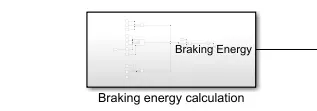
Fig: above model implemented as a subsystem that gives output of Braking energy

Similarly for Traction we implement the same way, just take care of the Velcity vector being fed for calculation.

important : Velocity should be those points where `(dV)/dt>0` for Traction power calculation

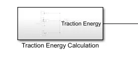
Fig: above model implemented as a subsystem that gives output of Traction energy

So this all is implemented as :

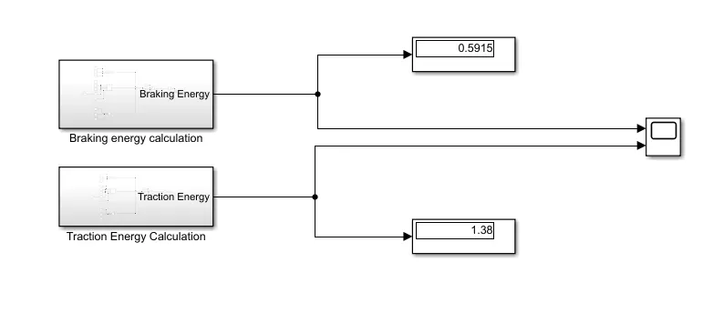
Fig: calculation of the Braking and Traction energy for the drive cycle

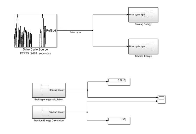
Fih: High level model of the complete system (top: takes the drive cycle and segments into Traction and Braking according to `(dV)/dt`) and below (implements the formula and integrates to calculate the corresponding energy)

Result: for the FTP75 drive cycle with driving time = 1400 s

total Traction energy = 1.38 kWhr

total Braking energy = 0.5915 kWhr

so the total energy required for braking is 0.5915 kWhr.

looking at the Energy plots we see the following result

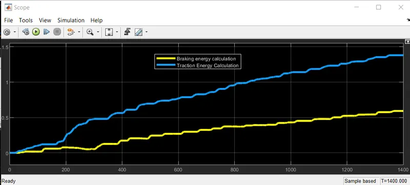
Fig: Traction Energy and Braking energy plotted together

Fig: this matches closely with the result we were expecting from the textbook picture of it for FTP75 drive cycle

so `=> "Braking Energy"/"Traction Energy" = 0.5915/1.38 = 42.86%`

------------------------------------------------------------------------------------------------------------------------------------------.

2. Why electric motor can’t develop braking torque at high speed similar to starting? How electric and mechanical brakes are coordinated?

Solution 2:

Braking torque developed by the motor is usuaslly not enough to fuflfill the desired Braking torque requirement of the vehicle.

Braking Torque of the vehicle deppends on 2 things:

1. Speed of the vehicle
2. Deceleration required, (how fast to stop the vehicle)

so in some cases ,below a thrshold the motor is able to generate the rewuired braking torque alone but after that it is required to use the mechanical brakes also since the torque requirement cannot be fuflfilled by the Motor.

Fig: usual torque-speed char of the EV ELectric motor

we see that at high speeds (`omega > omega_("base")`) the ,motor enters into the constant Power region and hence as `omega uparrow` the `tau downarrow` so the torque that is developed by the motor , high in the starting region is not what its provided at higher speeds since it is operating in the constant power region.

Coordination of the Electrical and Mechanical brakes:

The function of the vehicle brake system is to reduce the vehicle speed quickly while keeping
the vehicle traveling direction stable and controllable under various road conditions. These
requirements are satisfied by applying sufficient braking force on the wheels and properly
allocating the total braking force on the front and rear wheels.

the Maximum Braking force is limited by the Road-Wheel adhesive capability as

`=> F_("b max") = mu W`

this is also affected by the slip which is defined as:

`=> s = (1 - (romega)/V)xx100%`

the different forces acting on a vehicle on a flate road , after ignoring the Drag and Rolling resistance since they are negligible when compared to the braking forces

the deceleration of the vehicle will be as:

`=> j = (F_(bf) + F_(br))/M`

where `F_(bf)` and `F_(br)` is the braking force ofb the fromt and rear axles respectively.

also during braking there is a load transfer from the rear wheels to the front wheels,which are as `W_f` and `W_r` respectively

considering the the variables shown in the figure we can get the following relation :

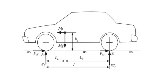
Fig: variables considered for derivation of the formulas

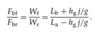
this is the relation between the 2 brake forces on the front and rear alxes.

substituting the value of j in the above eqaution we can derive the ideal brake force distribution curve.

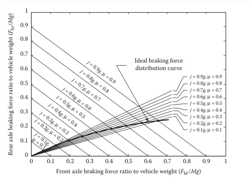
Fig: ideal brake force distribution curves for Rear and Front axles

when strong braking is required both the Rear and Front wheels obtain maximum Braking which is limited by the `mu` of the road. we have to limit the brake foce applied to avoid locking which is done with the activation of the ABS which prevents the brake force to get so high as to lock the wheels,

in that case the maximum deceleration rate is :

`=> j = (F_("br max") + F_("bf max"))/M` = `(W_f + W_r)mu/M = gmu`

following the ideal braking curve makes the system very complex since it is non linear hyperbolic in nature, so we instead use a fixed linear proportion which is defined by the ration of front braking force and total braking force

`=> beta = F_(bf)/F_(b)`

even though not fully followingt he ideal curve brake performance is good by the use of Electric braking systems(EBS)

we can easily get the Front and Reat brake force as

`=> F_(bf) = betaF_b`

`=> F_(br) = (1-beta)F_b`

`=>F_(bf)/F_(br) = beta/(1-beta)`

using the above equation and the other eqaution

we can get the actual brake force distribution curve:

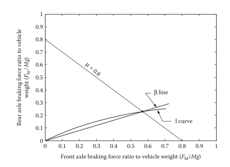
Fig: ideal and actual brake force distributionm curve

one very imortant safety consideration:

the front wheels should always lock before than the rear wheels.

if the rear wheels block first it will lead directional instability due to yaywing motion about the front wheel axis. in case of the Front wheel lockup first there is a motion too but unlike the rear wheel case it has a self-correcting moment due to the inertial force of the vehicle about the yaw center of the rear axle,

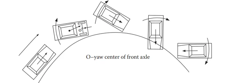
Fig: loss of directional stability due to lockup of rear wheels before the front wheels

This wheel lockup is detected using the sensors to meausre rotating speed of the wheels and prevent wheel lockup by reducing the brake force by reducing the pressure in the brake cyclinders by ABS

for the stable case: front wheel lock before rear wheel the `beta` line should be bleow the `I` line.

but also

when the `beta` line is much below the `I` line then in that case most of the braking force ois applied on the front wheel and after they are locked the rear wheels don not experience a high force and not able to use the total road adhesive capability to avaoid this braking reagulation are present to tell us the minimum amount of rear brake force to apply.

like te ECE brake regulation:

mathematically it states:

`=> F_(bf)/W_f >= F_(br)/W_r`

this makes sure that rear wheels are never locked before the front wheels.

the minimum braking force to be applied on the rear wheels is:

`=> j/g >= (0.1 + 0.85(mu - 0.2))`

what it means: when the front wheels are locked then the brake force applied on the rear wheel must be enough to produce a deceleration rate of not less than j

using all the eqautions we can get the following curve

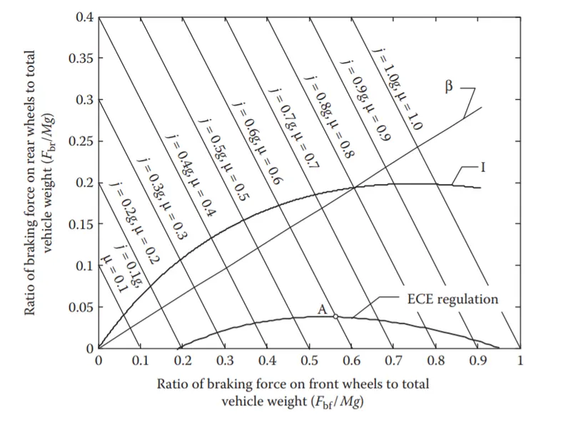
Fig: I curve , `beta` curve and ECE regulation curve for minimum rear brake force in one graph

the brake system should be such that the real braking force distribution lies in the area between the I curve and the ECE curve under all road conditions.

Cases:

Case I: front wheel locked, rear wheel not locked.

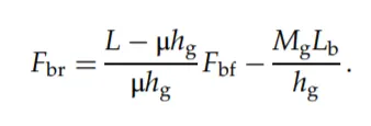
will generate a group of line (f lines) to represent the Front and Rear wheel braking force in this case.

Case II: front wheels not locked, rear wheels locked

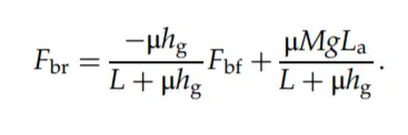
generates a gropu of other lines r lines

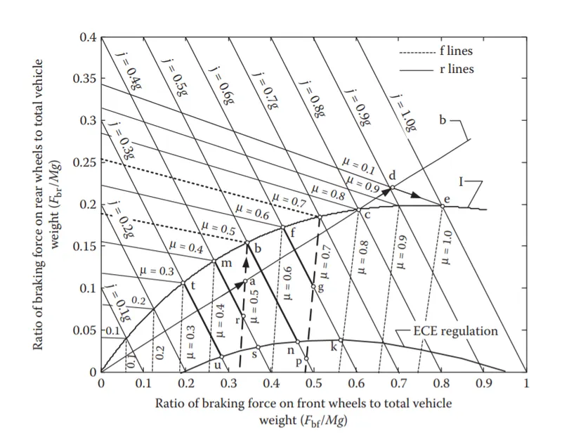
Fih: brake force analysis for different `mus`

Maximum available Brake force on the front wheels:

in EVs and HEVs motors are usually employed to driev te front wheels, which means that regen braking is only available in the front wheels, so in the braking system more energy should be allocated to the front wheels for max recovery of energy .

since we know that the motor is not capable of producing the high Brakign torque in some cases, we usually have a combination of thr meachnical and electrical braking in Evs

Most important considerations while designing the brake system:

1. how to distribute the total brkaing force among the front and rear so that we can get maximum energy regenerated but safely
2. how to distribute the forces on the front and rear axles to get stable braking perfromance

2 conifuration of the Hybrid Brake systems are possible:

1. Parrallel hybrid
2. fully controllable hybrid

electric motor will apply the braking to the front wheels depending upon the speed of the vehicle and the brake pedal position which will tell about the Braking strength required and the braking control strategy to employ which is embedded in teh vehicle controller

only electric braking is controlled by electronics and meachanical brake is controlled by the driver's brake pedal. Meachnical brakes do have elecronics which is employed when it is about to stop, ABS.

brake force allocation strategy:

• Meachanical brake has fixed brake force distribution as represented by the `beta` line
• total brake force = mechanical + electrical

case: when very low speed or near lockup (`omega < omega_("threshold")`)

no electric braking employed as the speed is very low so the EMF induced is not enough to generate a significant amount of energy. This is usually defined by a theshold. BElow this only the Mechanical braking is acting.

case: `omega>omega_("threshold")` and deceleration rate required can be fully fulfilled by the motor

no mechanical braking, only electric braking since it can fully provide the required Braking torque.

case: `omega>omega_("threshold")` and deceleration rate required can NOT be fully fulfilled by the motor and is not very high

now both regen and mechanical braking have to be used . Electric braking portion is associated with the power capacity of the motor and the energy storage.

case: when desired deceleration further increases than a value ,ex 0.6g, the elecric braking is gradually reduced to 0

this is important fos safety as it eill reduce the stopping distance and also provide strong mechanical braking.

all this is done to esnure that the braking distribution is closer to the ideal braking distribution curve.

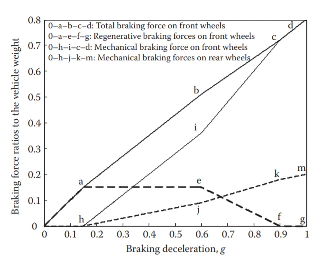
Fig: Different Brake force ratios (total, regen, meachanical on front and rear)

this can be seen as the mechanical + electrical plot in the belwo graph

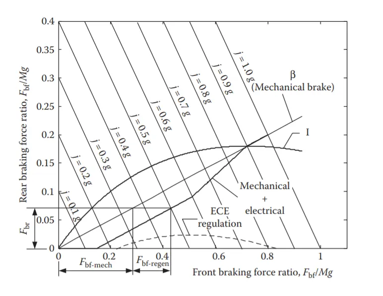
Fig: Hybrid brake system total brake force with I curve and `beta` curve

------------------------------------------------------------------------------------------------------------------------------------------.

3. Make a MATLAB program which plots contour of given motor speed, torque and efficiency values. Attach the code as a .m file attach a screenshot of all the plots.

one key objective of Electric vehicle is increasing the range of the vehicle for which it is very importnat to study the efficiency map of the motor so that we design a powertrain that operates in the maximum efficiecny zone as much as possible.

the efficiency primarilt depends on the speed and torque of the machine.After plotting the efficiency mnap we can find out how the powertrain operates and design it for optimized efficiency.

Also note that this is temperature dependent , as the tenperature of the machine increases, they lose energy more and become less efficient. therefore it is very crucial to keep the temperature within a specified limit.

may sound simple but this is only the efficiecny considering the Torque Speed spectrum of the machine while in practice it also depens on the gear ratio, temeperature and even Battery SoC. All these variables may lead to a several hundreds of scenarios for a single powertrain

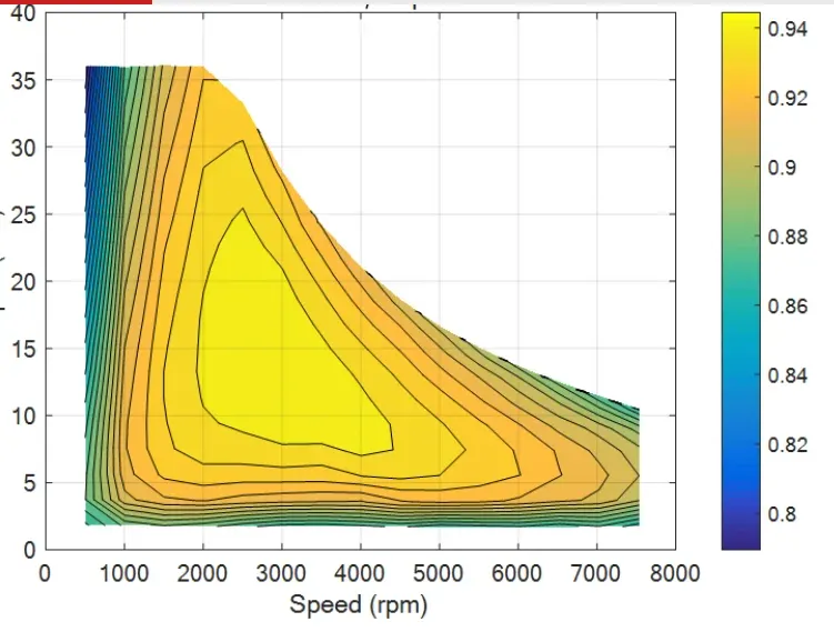
Fig: Efficiency map of a Motor used in a powertrain

I will be woking on the Efficiency plot of a Surface Permanent magnet AC Machine .

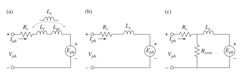
Fig: per phase equivalnet cricuit of SPM machine

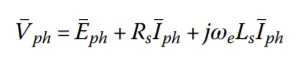
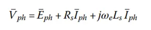
using phasor analysis we can come to the above equation.

we will be usign the direct axis or d-axis as the reference phasor.

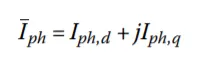
ther per pahse current `I_(ph)` can be resolved into 2 components as

It is useful to express the voltages in rectangular or Cartesian format as follows:

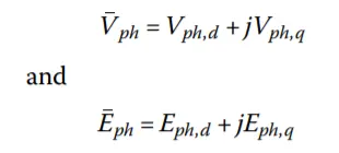
for the simplification of anaysis the Back EMF is considered to be only represented by the quadrature component.

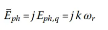
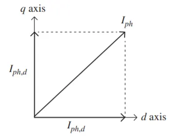
Fig: the d and q axis

we can represent the phasors in the motoring and generating mode ads below.Notice that the phase current anf back EMF are represented by the quadrature component only.

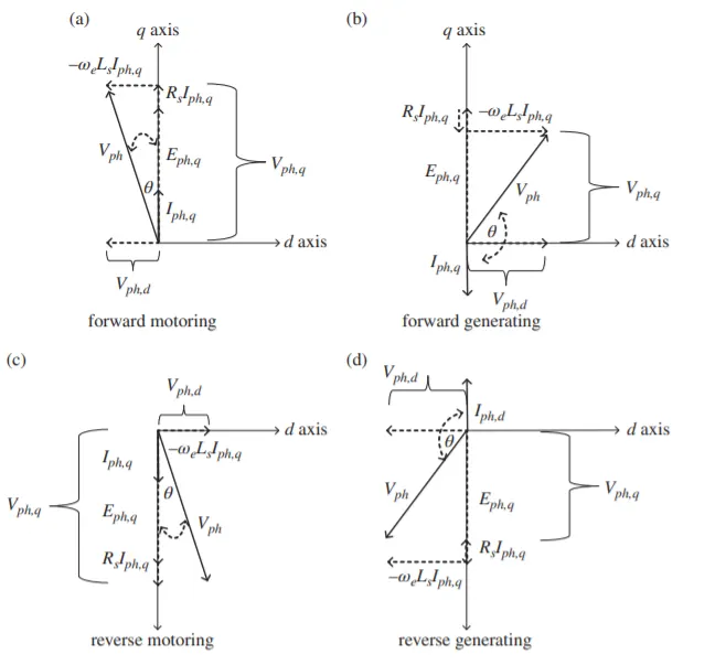
Fig: Phasor diagrams for the 4 modes of operation

When the SPM machine is motoring, the quadrature current is in phase with the back emf and is the torque-generating component of current. The direct or field component is aligned with the permanent magnet and lags the quadrature component by 90 .

WE SEE THAT:Iph,q and back emf Eph,q are in phase for motoring and 180 out of phase for generating as can be seen in the above phasor diagrams.

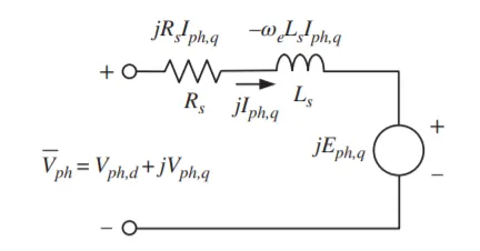
Fig: Phasor based Equivalent circuit of the SPM machine

also from the phasors we see that:

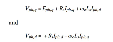
quadrature component of the supply voltage `V_(ph,q)` = sum of back emf `E_(ph,q)` and ohmic voltage drop across stator resistance `I_(ph,q)R_s`

direct component of supply voltage: is equal to drop across Synchronous resistance = `-omega_e L_sI_(ph,q)`

Also for below rated speed: there is no need for demagnitization to reduce the flux , so the Direct or Magnetizing current is zero for operation below rated speed.

therefore below rated speed `=>I_(ph,d) = 0`

so `=> I_(ph) = jI_(ph,q) = jT_(em)/(3k)`

so the volatge equation becomes

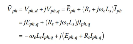
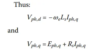
for calculating the power:

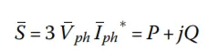
after solving the real power supplied to the machine is given by

where the 2nd term in the RHS is the stator copper loss and the 1st term is the Electromagnetic Power supplied to the machine .

if the no load torque is `T_(nl)` then the output rotor power is given by

`=> P_r = 3E_(ph,q)I_(ph,q) - T_(nl)omega_r`

the electromagnetic torque is: `T_(em) = 3kI_(ph,q)`

and the Rotor Torques is : `T_r = 3kI_(ph,q) - T_(nl)`

so the machine loss is given by:

`=>P_("loss") = 3R_sI_(ph,q)^2 + T_(nl)omega_r`

hence efficiency will be :

`=> eta = P_r/P *100% `

also in SPM unlike the IPM machine we see that the torque component due to the d-axis cancel out

and we ende up with the same expression we started with

`T_(em) = 3kI_(ph,q)`

in the `I_(ph)` the `I_(ph,q)` strenthens the flux while the `I_(ph,d)` weakens it.

subsituting the values in the equation

we end up with

the equivalent magnetizing current is due the permament magnet is `I_(ph,m)`, which can be found out using the bewlo equation

the current source to represen the magnet is

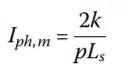
Cases for the magnetizing current

this above magnetizing current is the reference phasor for further analysis.

Below rated speed:

`=>E_(ph,q) = komega_r`

and `=>I_(ph,d) = 0 `

Above rated speed:

we control the value of the field current in such a way that the back emf at the presemnt operating speed is equal to the back emf at the rated speed.

`=>E_((ph,q)("rated")) = komega_("rated") = komega_r + p/2 omega_rL_sI_(ph,d)`

required field current is :

`=>I_(ph,d) = (2k)/(PL_s)(omega_(rrated)/omega_r - 1)= I_(ph,m)(omega_(rrated)/omega_r - 1)`

Applying the equations to plot the efficiency map/contours

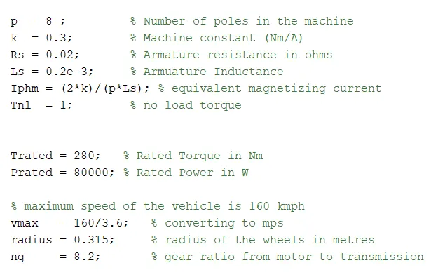
Fig: Motor parameters whoss efficiency map we are going to plot

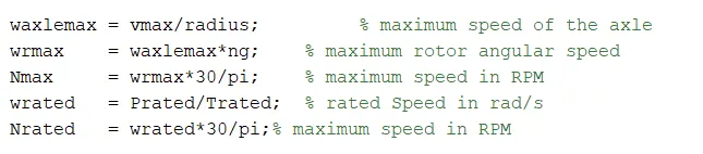
Fig: calculating the rated and maximum speed of the rotor

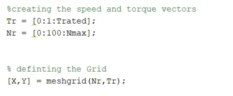
Fig: creating the speed and torque vectors and the meshgrid to get the XY graph limitis for the map

Fig: calculating the output power using the formula `=>P = Txx omega`

Fig: usinfg field weakening current(`I_(ph,q)`) only after the speed> rated speed

as we saw in the magnetizing current values for cases above abd below rated speed.

using the equation for `I_(ph,d)` above the rated speed that we saw and employing it here. which was

`=>I_(ph,d)= I_(ph,m)(omega_(rrated)/omega_r - 1)`

calculating the `P_("out")` as `P_("in") + P_("loss")`

as we saw in the derivation as

`=>P_("loss") = 3R_sI_(ph)^2 + T_(nl)omega_r`

and as `=>I_(ph) = I_(ph,q) + I_(ph,d)`

`=>P_("loss") = 3R_sI_(ph,q)^2 + 3R_sI_(ph,d)^2 + T_(nl)omega_r`

so `=>P_("in") = P_("out") + P_("loss")`

which is implemented as :

=>P_("in") = P_("out") + 3R_sI_(ph,q)^2 + 3R_sI_(ph,d)^2 + T_(nl)omega_r`

after substituing thje value of `P_("loss")` in the formula in the MATLAB code

Fig: implementing the formula derived above for `P_("out")` in code and `eta = P_("out")/P("in")`

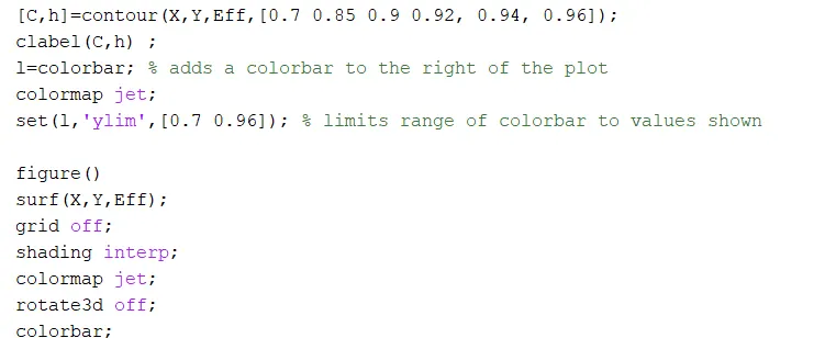
Fig: code to plot the contour of efficincy plot and also the surface for complete region

note: efficiency plots for `eta = 70,85,90,92,94,96 %` has been calculated

Resulting plots:

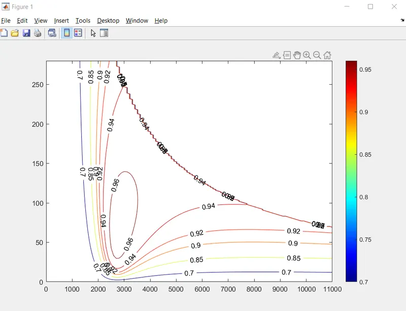
Fig: contour plot for the given efficeincies plotted with corresponding colorbar

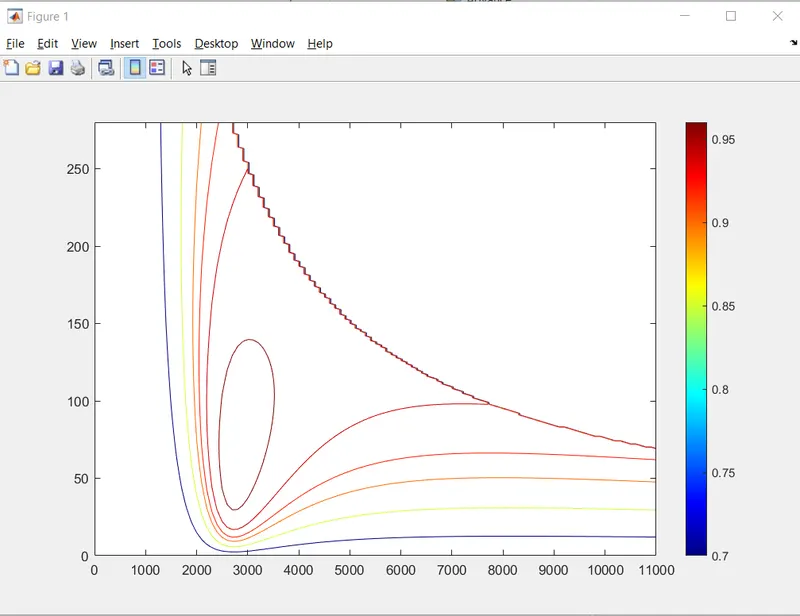
Fig: removing the contour line values for better visualization . efficiency Contour map of out SPM AC machine

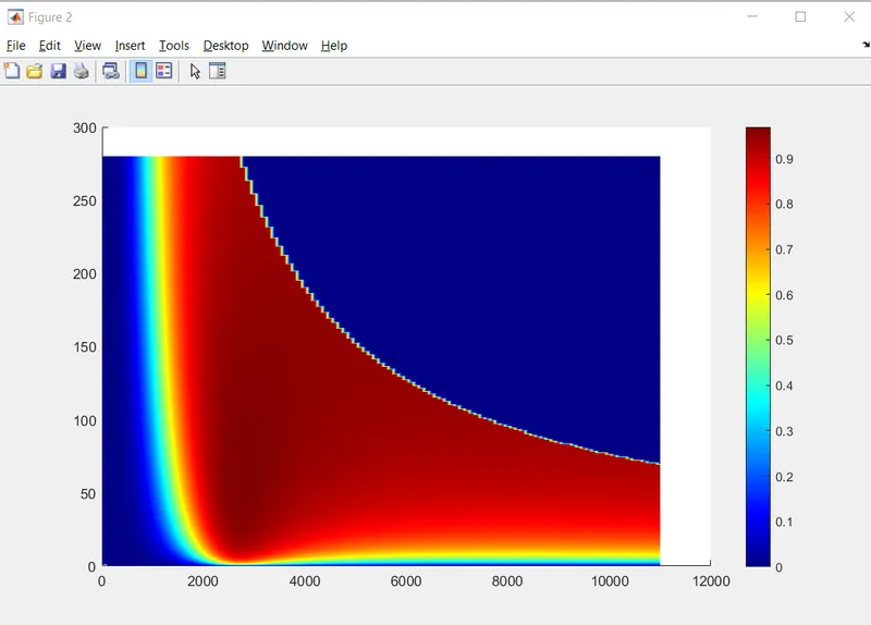
Fig: Efficiency map of the machine for complete Speed-Torque range of the opeartion. Colorbar to get the values of efficiency at a point

Fig: we see the Efficiency map is similar to what we would expect for the motor(colors different as i personlly perfer jet colormap but color limits can bee seen as similar on the colorbar)