Week-11 Challenge: Braking

Driving Cycle:-Driving cycle consists of a sequence of several vehicles operating conditions (idle, acceleration, cruise and deceleration) and is considered as a signature of driving characteristics of that city or region. The driving pattern varies from city to city and from region to region. Consequently, the driving cycles developed in a certain region may not be a good representation elsewhere unless the driving characteristics are conspicuously similar.

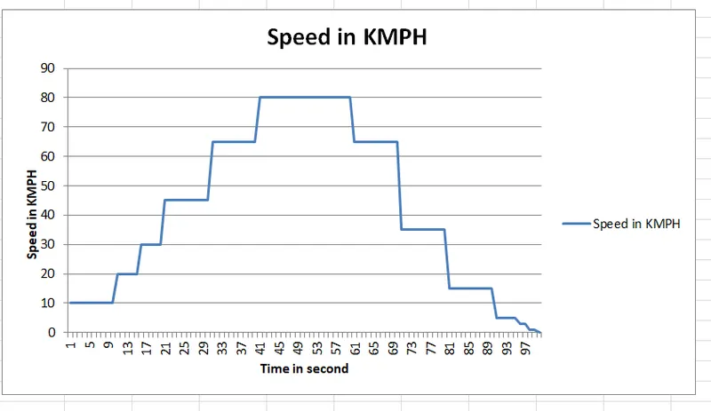
Fig 1 :-Graph of Speed vs Kmph in Indian road

`Braking Power= 1 div 2 (mass x velocity ^2)`

mass=Mass of vehicle+Mass of fuel

Velocity=(final velocity-initial velocity)

`onsider now initial velocity is 9 kmph and final velocity is 49 Kmph `

Mass of vehicle will be 1500 Kg and mass of fuel will of around 35 kg the equation will become as

`Braking Power=1 div 2 *(1500+35)*(45-9)`

`Braking power=1 div 2 *(1535)*(36)`

`Braking power=6885 J`

or

`Braking power=6.85KJ`

2

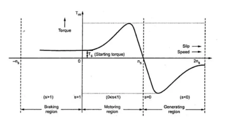
Fig2:-Speed torque of induction motor

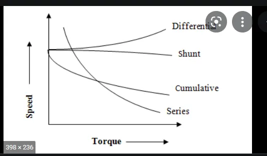
Fig3:Speed and torque of DC motor

Now in the above case, they ate 2 casers once at the starting we are going to get more torque in both cases. if you were going to accelerate it can be getting sufficient torque. But at the time of applying Brake that time motor will be there in Regenerative mode and the torque will be there in negative torque and it is not in the positive quadrant and it cannot be reversed. In the dc machine, it cannot be determined and it comes in a negative Quadrant and it cannot be as much as a positive quadrant. and the reason it will be there in negative mode.

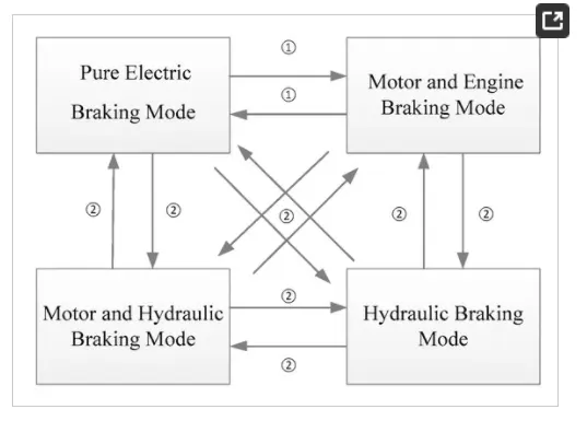
Fig4:Diffent type of Brakes at Electric Motor

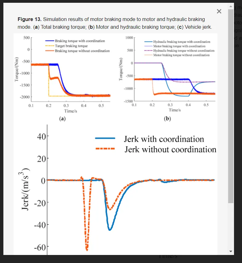
Fig5:-Brakes with coordination

hereinabove is a graph which will show both brakes with coordination.

Fig 5 will show the that too in blue colour with coordination.And in orange colour will show without coordination.

So it would be clear that both will work only if they were working fine.

3 contour layout

w=linspace(0,300,100);
T=linspace(0,2000,100);
kc=0.17;
ki=0.006;
kw=0.000015;
[X,Y]=meshgrid(w,T);
cu_losses=(Y.^2)*kc;
Fe_losses=X*ki;
windage_losses=(X.^3)*kw;
k=18;
output_power=X.*Y;
input_power=(cu_losses)+(Fe_losses)+(windage_losses)+(output_power)+k;
effy=(output_power)/(input_power);
n=linspace(1.0,2.0,10);
contourf(X,Y,effy,n);

output will be as shown below

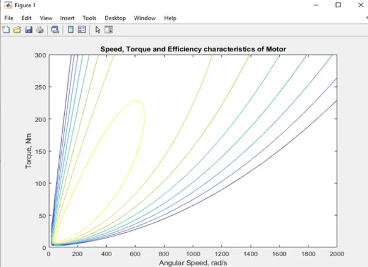
Fig 6:-Output of contour layout

it's basically a line that will follow all of the common points in the graph.

now in this example, we had given some constant values such as Kc, ki and K are constant and KT were given

SO from them, we are getting Input Power, output power.

and we had put contour to get output.

Result:-

• The driving cycle will be discussed and we had taken an example of the Indian drive cycle and braking power is calculated.
• The reason for less torque can be determined and how mechanical and electric power is known.
• The contour layout is plotted and the reason is discussed.