Week-11 Challenge: Braking
>Objective:
- For a defined driving cycle, calculate the energy required for braking.
- Why electric motor can’t develop braking torque at high speed similar to starting? How electric and mechanical brakes are coordinated?
- Make a MATLAB program which plots contour of given motor speed, torque and efficiency values. Attach the code as a .m file attach a screenshot of all the plots.
- 1.For a defined driving cycle, calculate the energy required for braking.
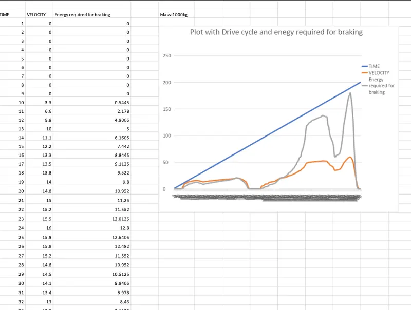
Consider speed-torque characteristics of a motor used in EV application
An EV can achieve high speed during starting but can't achieve the same with the same speed during braking. This is true in the EV motor case.
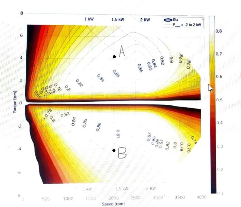
During low speed, the torque produced by the motor is almost constant and the motor operates in the constant torque region. Thus it has higher acceleration power. Now consider the point A in the above characteristics of a motor with a vehicle speed of 100 mph at that point which is in a constant power region.
Now when it comes to the braking part where torque is negative, Let's consider the replicate of point A is point B and the braking torque is at point B is around -4 N-m compared to peak torque of -7 N-m.
The peak acceleration torque and peak deceleration torque is not the same for a motor, i.e at the low speed we get high torque and at high speed, the value of torque is lower. So we cannot say that the motor which is producing 7 N-m of torque for acceleration can also produce -7 N-m of braking torque. so because we are operating the braking torque at field weakening region or operating the motor abovr base speed we must also know that the torque value is compromised or lower.
The braking torque of EV motor is not high as acceleration torque. Therefore regenerative braking cannot happen so effectively such that all power produced is pulled back to the battery.
This is one of the motor limitations.
The electric and mechanical brakes are coordinated in two different ways.
1. Series brake control strategy
2. Parallel brake control strategy.
In a series brake control strategy, we apply the mechanical brake and regenerative electrical brake one after another, i.e we apply only one brake at a time (either mechanical braking or regenerative braking).
In parallel brake control, we apply both brakes simultaneously.
The series has two classifications.
(a) Comfort of driver
(b) Energy efficiency.
Electric Driven Intelligent Brake (EDIB)
It is a braking strategy developed in Nissan Leaf.
This EDIB is a combination of a hydraulic brake along with a regenerative brake
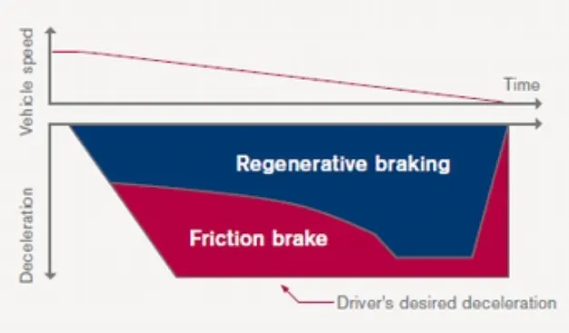
Here parallel braking technique is used initially. At higher braking speed, we have both regenerative braking and frictional braking and whenever the speed of the vehicle reduces at the low speed we get higher torque by the motor, and percentage sharing for regenerative braking increases in lower speed.
3.Make a MATLAB program which plots contour of given motor speed, torque and efficiency values. Attach the code as a .m file attach a screenshot of all the plots.
- Iron loss: This is defined as the loss that is caused due to the alternating flux in the core of the transformer. As the loss occurs in the core, therefore iron loss is also known as core loss. There are two types of iron losses, and they are eddy current loss and hysteresis loss.(KFe-t2)
- Copper loss: This is defined as the heat that is produced by the electrical currents in the conductors of transformer windings. It is an undesirable transfer of energy resulting from the induced currents in the adjacent components.(Kcu*w^2)
- Windage loss is the reduction in efficiency due to windage forces. For example, electric motors are affected by friction between the rotor and air. (Kw*T^3)
-
Constant losses: denoted a C
Total losses = (Kcu*w^2)+ (KFe-t2) + (Kw*T^3) + C
MATLAB CODE:
clear all
close all
clc
% Speed Array
omega = linspace(0, 300, 100);
% Torque Array
T = linspace(0, 2000, 100);
% Meshgrid
[X,Y] = meshgrid(T, omega);

% Loss Coefficients
cu = 0.17;               % Copper coefficient
fe = 0.006;              % Iron coefficient
win = 0.000015;          % Windage coefficient

% Losses
cu_loss = cu*(Y.^2);     % Copper Losses
fe_loss = fe*(X.^2);     % Iron Losses
win_loss = win*(X.^3);   % Windage Losses
cond_loss = 18;          % Conduction Losses

% Output Power
P_out = (X.*Y);
% Input Power
P_in = P_out + (cu_loss) + (fe_loss) + (win_loss) + (cond_loss);
% Efficiency
n = ((P_out)./(P_in));

% Efficiency values for contour
W = linspace(0.75, 0.95, 10);
% Contour Plot
contour(X,Y,n,W)
xlabel('Angular Speed, rad/s')
ylabel('Torque, Nm')
title('Speed, Torque and Efficiency characteristics of Motor')
>OUTPUT:
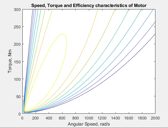
From this plot contour observation, we can see that the highest level of efficiency arises in the innermost contour plot
Were the efficiency decreases the alternative the contour increases in the size of the contour