Week-11 Challenge: Braking

AIM: Study the Brake Energy concept and calculate required energy for braking.

OBJECTIVES:

• Calculate the energy required for braking for a defined drive cycle.
• Discuss hoe the electric and mechanical brakes are co-related.
• Prepare a MATLAB script to plot a Contour of given motor speed, torque and efficiency.

1. For a defined driving cycle, calculate the energy required for braking.

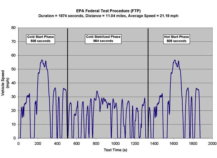
A drive cycle is typically represented by a series of data points which plots vehicle speed against time. Driving cycles are produced to assess the performance of vehicles in various ways, including fuel consumption and pollutant emissions.

Main uses of driving cycles are

• To assess the performance of a vehicle (fuel economy, emission tests)
• To analyse battery state and energy consumption in Electric vehicles
• To simulate vehicle model prior to the actual development

The EPA Federal Test Procedure, commonly known as FTP-75 for the city driving cycle, are a series of tests defined by the US Environmental Protection Agency (EPA) to measure tailpipe emissions and fuel economy of passenger cars (excluding light trucks and heavy-duty vehicles).

The Kinetic energy of the moving car will give out required Braking energy to control the vehicle.

KE = ½ * M*V²

Were M = Mass of the vehicle = 1000 kg

V = Velocity of the vehicle mph

The deceleration from V1 to V2 will reduce the energy. This energy is being saved in hybrid and electrical cars as regenerative energy.

The linear energy change is equal to:

KE linear change = ½ * M * (V₁^{2 –} V₂²)

However, because of moment of inertia of the wheels compared to the mass of the car, the contribution of the wheel's change of energy is not significant.

MATLAB program to calculate the Braking energy required to control the vehicle for a standard drive cycle (Federal Test Procedure)

clear all
close all
clc

% Load the Drive cycle data file
load ftpdrivecycle.mat;
time = ftpdrivecycle.Time;
Velocity = ftpdrivecycle.Speed;
Mass = 1000;    % Mass of the vehicle

for i = 1:1874
    if Velocity(i) > Velocity(i+1)
        Braking_Energy(i) = 0.5*Mass*Velocity(i)^2;
    else Braking_Energy(i) = 0;
        sum(Braking_Energy);
    end
end

figure(1)
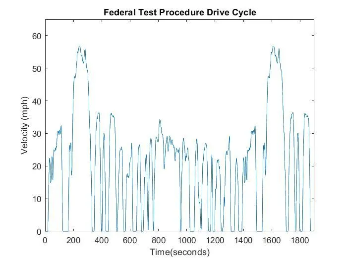
plot(time,Velocity)
axis([0 1900 0 65])
xlabel('Time(seconds)')
ylabel('Velocity (mph)')
title('Federal Test Procedure Drive Cycle')

figure(2)
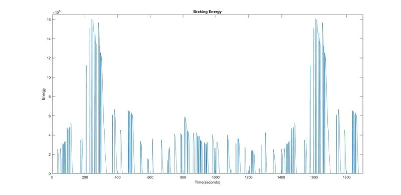
plot(Braking_Energy)
axis([0 1900 0 1650000])
xlabel('Time(seconds)')
ylabel('Energy')
title('Braking Energy')
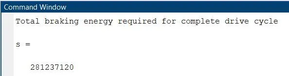
disp('Total braking energy required for complete drive cycle')
s = sum(Braking_Energy)

Code Explanation

• I have considered the Standard Federal Test Procedure (FTP) drive cycle to find out the braking energy required.
• Loaded the file and separated the variable of Time and Speed in to matrix form.
• By using the Kinetic energy equation, the required braking energy is calculated.
• Two plots we plotted i.e., Velocity Vs Time and Energy Vs Time and the total energy required for braking is 281237.120 Kw

OUTPUT PLOTS:

Braking Enegry

2. Why electric motor can’t develop braking torque at high speed similar to starting? How electric and mechanical brakes are coordinated?

Electric motor has high torque producing capability at low starting speed. But as the speed increases the torque values rapidly decreases.

Starting Torque - During the starting stage, the speed values are low and thus torque produced is much high.

Braking Torque - In the braking stage, the speed of the motor is of very high value and sometimes greater the synchronous speed values, thus due to high-speed values the braking torque generated will be a low value only.

Factors limiting the braking power generated during regenerative braking

(a) Braking power is not only limited by the motor's power rating, but by the charging power limit of the battery pack. This limit depends on the battery type (chemical composition) and changes with temperature.

(b) The kinetic energy of a slowly moving car is low enough that very little energy is put back into the battery as the car comes to a stop. In fact, the last little bit of slowing the vehicle down generates such a small amount of energy that it does not even cover the fixed losses in the inverter and motor.

(c) Regenerative braking is necessarily limited when the batteries are fully charged. Because the additional charge from regenerative braking would cause the voltage of a full battery to rise above a safe level, the motor controller will limit regain torque in this case.

Coordination of electric and mechanical braking

Generally Electric motor don’t have high torque capacity to handle all of the vehicle braking. Hence during the initial braking time, mechanical brakes are used in larger proportion than regenerative braking.

Once the braking torque value starts to decrease the regenerative braking is increased in proportion.

Basically, there are three different brake control strategies:

• series braking with optimal braking feel
• series braking with optimal energy recovery
• parallel braking

Series Braking with Optimal Braking Feel

• The control objective is to minimize the stopping distance and optimize the driver’s feel.

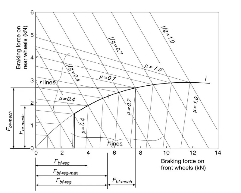
When the commanded deceleration (represented by the braking pedal position) is less than 0.2g, only the regenerative braking on the front wheels is applied, which emulates the engine retarding function in conventional vehicles.

When the commanded deceleration is greater than 0.2g, the braking forces on the front and rear wheels follow the ideal braking forces distribution curve I, as shown in Figure by the thick solid line.

The braking force on the front wheels (driven axle) is divided into two parts: regenerative braking force and mechanically frictional braking force.

When the braking force demanded is less than the maximum braking force that the electric motor can produce, only electrically regenerative braking will apply.

When the commanded braking force is greater than the available regenerative braking force, the electric motor will operate to produce its maximum braking torque, and the remaining braking force is met by the mechanical brake system.

It should be noted that the maximum regenerative braking force produced by an electric motor is closely related to the electric motor’s speed.

At low speed (lower than its base speed), the maximum torque is constant.

However, at high speed (higher than its base speed), the maximum torque decreases hyperbolically with its speed.

Therefore, the mechanical brake torque at a given vehicle deceleration varies with vehicle speed.

Series Brake - Optimal Energy Recovery

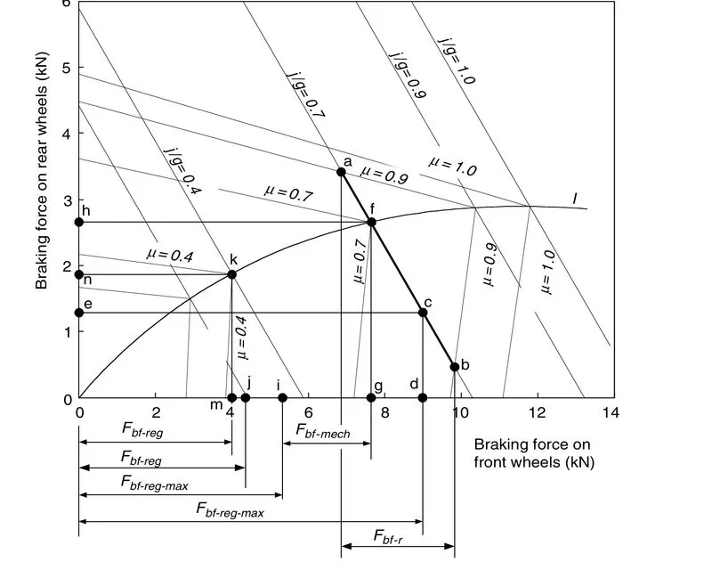
The principle of the series braking system with optimal energy recovery is to recover the braking energy as much as possible in the condition of meeting the total braking force demanded for the given deceleration.

(a) When the vehicle is braked with an acceleration rate of j /g < μ, the braking forces on the front and rear wheels can be varied in a certain range. This variation range of the front and rear axles is shown in figure by the thick solid line ab, where μ =0.9 and j/g = 0.7. In this case, regenerative braking should be used in priority.

If the available regenerative braking force (maximum braking force produced by the electric motor) is in this range (point c in Figure, for example), the braking force on the front wheels should be developed only by regenerative braking without mechanical braking. The braking force on the rear wheels, represented by point e, should be developed in order to meet the total braking force requirement.

If, on the same road, the available regenerative braking force is less than the value corresponding to point a (e.g., Figure: Demonstration of series braking — optimal energy recovery [1] point i in Figure), the electric motor should be controlled to produce its maximum regenerative braking force. The front and rear braking forces should be controlled at point f so as to optimize the driver feel and reduce braking distance. In this case, additional braking force on the front wheels must be developed by mechanical braking, and the braking force on the rear axle is represented by point h.

(b) When the commanded deceleration rate, j/g, is much smaller than the road adhesive coefficient (j /g = 0.3 in Figure 2 for example), and the regenerative braking force can meet the total braking force demand, only regenerative braking is used without mechanical braking on the front and rear wheels (point j in Figure).

(c) When the commanded deceleration rate, j/g, is equal to the road adhesive coefficient μ, the operating point of the front and rear braking forces must be on the curve I. On a road with a high adhesive coefficient (μ = 0.7, operating point f, in Figure, for example), the maximum regenerative braking force is applied and the remaining is supplied by the mechanical brake. On a road with a low adhesive coefficient (μ = 0.4, operating point k, in Figure, for example), regenerative braking alone is used to develop the front braking force.

(d) When the commanded deceleration rate, j /g, is greater than the road adhesive coefficient μ, this commanded deceleration rate will never be reached due to the limitation of the road adhesion. The maximum deceleration that the vehicle can obtain is (a / g) max = μ. The operating point of the front and rear braking forces is on the curve I, corresponding to μ (μ = 0.4 and j /g = 0.4 in Figure, for example); the operating point is pointing k and the maximum deceleration rate is j/g = 0.4. It should be noted that the series brake with both optimal feel and energy recovery needed active control of both electric regenerative braking and mechanical braking forces on the front and rear wheels. At present, such a braking system is under research and development.

Parallel Brake

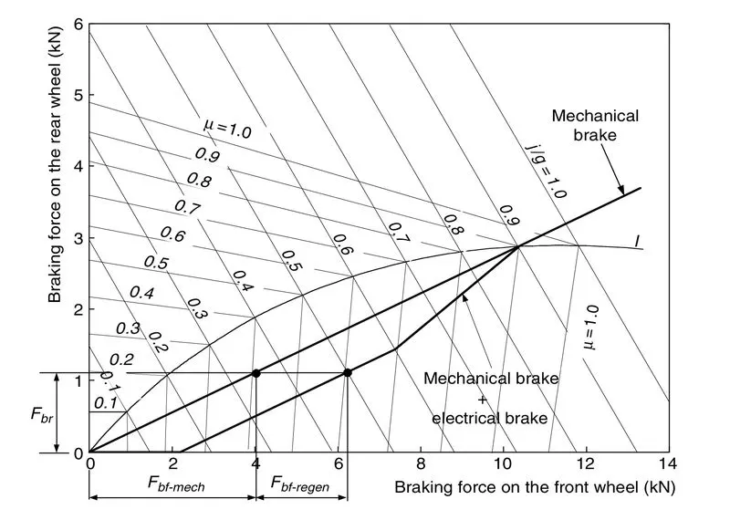
The parallel brake system includes both an electrical (regenerative) brake and a mechanical brake, which produce braking forces is parallel and simultaneously. The operating principle is illustrated in Figure, in which regenerative braking is applied only to the front wheels.

The parallel brake system has a conventional mechanical brake which has a fixed ratio of braking force distribution on the front and rear wheels. Regenerative braking adds additional braking force to the front wheels, resulting in the total braking force distribution curve. The mechanical braking forces on the front and rear axles are proportional to the hydraulic pressure in the master cylinder.

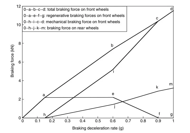
The regenerative braking force developed by the electric motor is a function of the hydraulic pressure of the master cylinder, and therefore a function of vehicle deceleration. Because the regenerative braking force available is a function of motor speed and because almost no kinetic energy can be recovered at low motor speed, the regenerative braking force at high vehicle deceleration (e.g., a /g = 0.9) is designed to be zero so as to maintain braking balance.

When the demanded deceleration is less than this deceleration, regenerative braking is effective. When the braking deceleration commanded is less than a given value, say 0.15g, only regenerative braking is applied. This emulates the engine retarding in a conventional vehicle. In Figure, the regenerative braking force, and mechanical braking forces on the front and rear wheels, Fbf mech and Fbr, are illustrated.

Above shown Figure shows the total braking force, regenerative braking force, and mechanical braking force on the front wheels as well as the braking force on the rear wheels in the parallel braking system of a passenger car. The parallel braking system does not need an electronically controlled mechanical brake system. A pressure sensor senses the hydraulic pressure in the master cylinder, which represents the deceleration demand. The pressure signal is regulated and sent to the electric motor controller to control the electric motor to produce the demanded braking torque.

Compared with the series braking of both optimal feel and energy recovery, the parallel braking system has a much simpler construction and control system. However, the driver’s feeling, and amount of energy recovered are compromised.

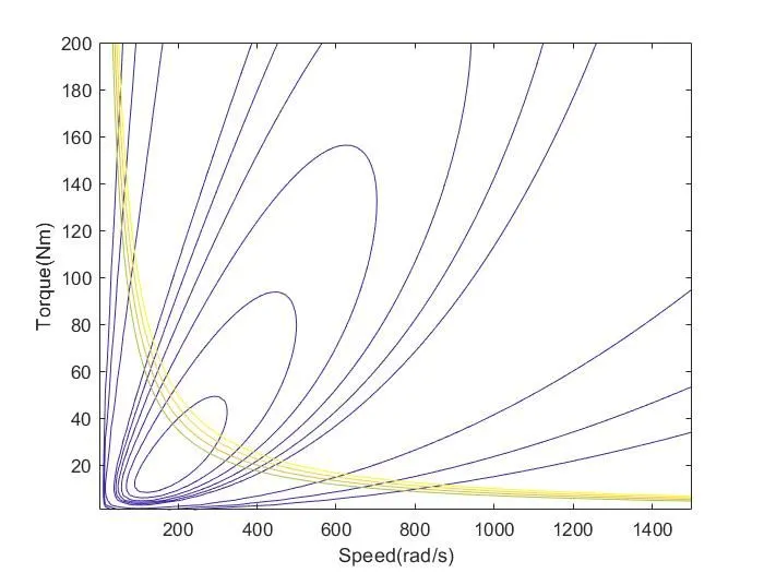
3.Make a MATLAB program which plots contour of given motor speed, torque and efficiency values. Attach the code as a .m file attach a screenshot of all the plots.

For any system there will be some losses, here in the motor there are three losses

• Copper losses
• Iron (Magnetic) losses
• Windage (Mechanical or Frictional) losses

For finding the values for these losses we need to conduct lot of experiments.

Output Power = Torque * Speed

Input power = Output Power + Kc + Ki + Kw + Motor constant

Efficiency = Output Power / Input power

MATLAB Program

% Program for finding Efficiency contour for electric motor
clear all
close all
clc

% Initialy set up the arrays for range
x = linspace(1,1500);   % speed,N.B rad/s
y = linspace(1,200);    % Torque N-m

% Define the Motor losses constants
kc = 0.2;   % copper losses
ki = 0.008; % iron losses
kw = 0.00001;   %windage losses
ContML = 20;    % motor constant losses
% Now make mesh to fins out the power 
[X,Y] = meshgrid(x,y);
Output_power = (X.*Y);  % Power = Torque*Speed

P = (Y.^2)*kc;  % copper losses
Q = X*ki;       % iron losses
R = (X.^3)*kw;  %windage losses
Input_power = Output_power + P + Q + R + ContML;
Efficiency = Output_power./Input_power;

% Now set the efficiency points , where the contour will be plotted
V = [0.60,0.7,0.80,0.90,0.91,0.92,0.93,0.94,0.95];
box off
grid off
contour(X,Y,Efficiency,V);
xlabel('Speed(rad/s)');
ylabel('Torque(Nm)');
hold on

% Now plot a contour of the Output power
V = [7000,8000,9000,10000];
contour(X,Y,Output_power,V);

OUTPUT PLOT:

Finally, the contour plot is drawn for required efficiency values. Efficiency decreases as we move away from the middle contour.

CONCLUSION:

Hence, we have studied the concept of Brake energy

• The total energy required for braking for a Federal Test Procedure (FTP) drive cycle is 281237.120 Kw
• Completely discussed how the electric and mechanical brakes are co-related.
• Prepared a MATLAB script to plot a Contour of given motor speed, torque and efficiency.

REFERENCE:

https://www.epa.gov/vehicle-and-fuel-emissions-testing/dynamometer-drive-schedules

Drive Link:

https://drive.google.com/drive/folders/1-p7kMy2fl3eiJRS4RqjrmPffJ5yx1UoJ?usp=sharing