Week-11 Challenge: Braking

AIM:

To explain the following,

• For a defined driving cycle, calculate the energy required for braking
• Why electric motor can’t develop braking torque at high speed similar to starting? How electric and mechanical brakes are coordinated?
• Make a MATLAB program which plots contour of given motor speed, torque and efficiency values. Attach the code as a .m file attach a screenshot of all the plots

OBJECTIVES:

• Explain the requirement with the detailed data
• Ensure using parameters for the calculation
• Create the matlab program and make a contour plot of it

1. For a defined driving cycle, calculate the energy required for braking

Driving Cycle:

• Driving cycles are consisting of an unique profile of stopping, starting, idling, constant speed cruising, acceleration and deceleration with a prescribed time frame, vary considerably worldwide, depending on specific traffic and road conditions

Main uses of driving cycles are,

1. To assess the performance of a vehicle (fuel economy, emission tests)
2. To analyze battery state and energy consumption in Electric Vehicles
3. To simulate vehicle model prior to the actual development

• The driving cycle is performed on a chassis dynamometer, where tailpipes emissions of the vehicle are collected and analyzed to assess the emissions rates
• In commercial vehicles area, the driving cycle is not performed on a vehicle dynamometer but on an engine dynamometer and is evaluated through a set of engine torque and speed points instead of vehicle speed points

Driving cycles can be classified as,

1. Model Driving Cycles
2. Transient Driving Cycles

Model Driving Cycle

• The model driving cycle comprises constant speed and does not represent a real driving pattern of a vehicle
• These driving cycles will be used for specific applications such as an emission test

Total distance : 11.023 kms

Total time : 1180 secs

Average speed : 33.6 kmph

2. Transient Driving Cycle

• The transient driving cycle represents an actual pattern of a vehicle which contains acceleration, deceleration, constant speed, etc
• Federal Test Procedure (FTP 75) is an example of a Transient Driving Cycle

Total distance : 17.77 kms

Total time : 1874 secs

Average speed : 34.1 kmph

Calculation of Energy Required for Braking:

• Governing formula: `E=1/2mv^2`

where,

E = Energy (`J`)

m = Mass of the vehicle (`Kg`)

v = Velocity of the vehicle (`m/s^2`)

`v_f`= Final velocity

`v_i`= Initial velocity

Therefore, `E=1/2m(v_f-v_i)^2`

Data:

Mass, m = 1000 Kgs

Run Time = 77 Secs

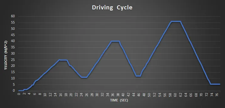
Total energy used for braking = `E_1+E_2+E_3`

Case-1

`E_1=1/2*m*(v_f-v_i)^2`

`=1/2*1000*(25-10.9)^2`

`=500*14.1^2`

`E_1=99405` J

Case-2

`E_2=1/2*m*(v_f-v_i)^2`

`=1/2*1000*(40-12.07)^2`

`=500*27.93^2`

`E_2=390042` J

Case-3

`E_3=1/2*m*(v_f-v_i)^2`

`=1/2*1000*(56-5.45)^2`

`=500*50.55^2`

`E_3=1277651` J

• Therefore, Total energy applied for the overall braking,

`E=E_1+E_2+E_3`

=99405+390042+1277651

E = 1767098 J (or) 1767.09 kJ

2. Why electric motor can’t develop braking torque at high speed similar to starting? How electric and mechanical brakes are coordinated?

Braking Torque:

• Generally, the braking torque required is much larger than the torque that an electric motor can produce. In EVs and HEVs, mechanically frictional braking systems must coexist with electrically regenerative braking. Thus, the proper design and control of both mechanical and electrical braking systems are major concerns
• The brake pad is pressed against the brake plate, thus developing a frictional torque on the brake plate. This braking torque results in a braking force in the tire–ground contact area. It is just this braking force that tries to stop the vehicle. The Braking Torque (`T_b`) is the moment of braking force about the center of rotation. The braking force can be expressed as

`T_b=F_b*R_d`

Where,

`T_b=` Braking Torque

`R_d=` Disc Radius

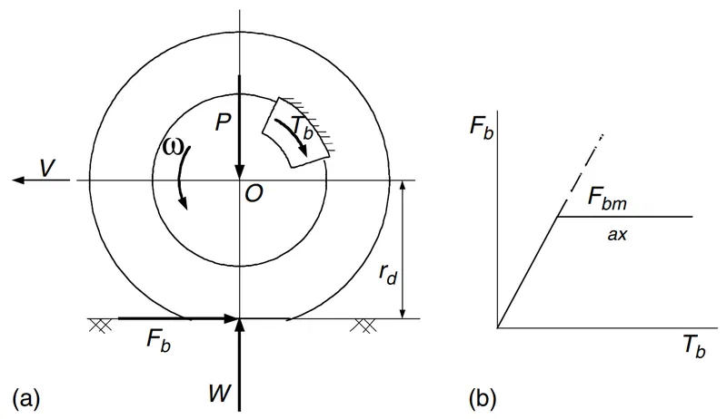
• The braking force increases with an increase in braking torque. However, when the braking force reaches the maximum braking force that the tire–ground adhesion can support, it will not increase further, although the braking torque may still increase. This maximum braking force limited by the adhesive capability can be expressed as

`F_(b max)=mu_bW`

• Here the electric motor can’t develop the braking torque at high speed due to the loss of energy there is no emf induced during the torque braaking

Coordination of Electric and Mechanical Brakes:

• Regenerative braking takes place whenever the speed of the motor exceeds the synchronous speed. This baking method is called regenerative baking because here the motor works as generator and supply itself is given power from the load like motors
• It is a form of braking in which the kinetic energy of the motor is returned to the power supply system. This type of braking is possible when the driven load forces the motor to run at a speed higher than its no-load speed with a constant excitation
• The motor back emf Eb is greater than the supply voltage V, which reverses the direction of the motor armature current. The motor begins to operate as an electric generator
• It is very interesting to note that regenerative braking cannot be used to stop a motor but to control its speed above the no-load speed of the motor driving the descending loads
• The main criteria for regenerative braking is that the rotor has to rotate at a speed higher than synchronous speed, only then the motor will act as a generator and the direction of current flow through the circuit and direction of the torque reverses and braking takes place
• The only disadvantage of this type of braking is that the motor has to run at super synchronous speed which may damage the motor mechanically and electrically, but regenerative braking can be done at sub synchronous speed if the variable frequency source is available
• Basically, there are two different brake control strategies, they are

1. Series braking
2. Parallel braking

1. Series Braking:

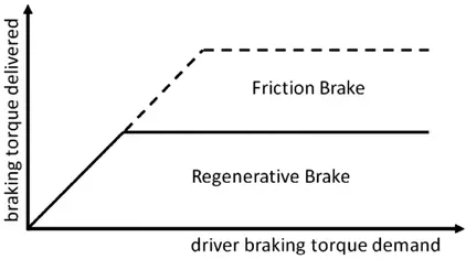
• The control objective is to minimize the stopping distance and optimize the driver’s feel. When the commanded deceleration (represented by the braking pedal position) is less than the required, only the regenerative braking on the front wheels is applied, which emulates the engine retarding function in conventional vehicles
• When the commanded deceleration is greater than the required, the braking forces on the front and rear wheels follow the ideal braking forces. The braking force on the front wheels (driven axle) is divided into two parts: regenerative
  braking force and mechanically frictional braking force
• When the braking force demanded is less than the maximum braking force that the electric motor can produce, only electrically regenerative braking will apply
• When the commanded braking force is greater than the available regenerative braking force, the electric motor will operate to produce its maximum braking torque, and the remaining braking force is met by the mechanical brake system
• It should be noted that the maximum regenerative braking force produced by an electric motor is closely related to the electric motor’s speed. At low speed (lower than its base speed), the maximum torque is constant
• However, at high speed (higher than its base speed), the maximum torque decreases hyperbolically with its speed. Therefore, the mechanical brake torque at a given vehicle deceleration varies with vehicle speed
• It should be noted that the series brake with both optimal feel and energy recovery has needed active control of both electric regenerative braking and mechanical braking forces on the front and rear wheels. At present, such a braking system is under research and development

2. Parallel Braking:

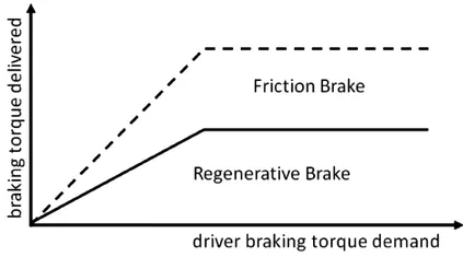
• The parallel brake system includes both an electrical (regenerative) brake and a mechanical brake, which produce braking forces is parallel and simultaneously
• The parallel brake system has a conventional mechanical brake which has a fixed ratio of braking force distribution on the front and rear wheels. Regenerative braking adds additional braking force to the front wheels, resulting in the total braking force distribution curve
• The mechanical braking forces on the front and rear axles are proportional to the hydraulic pressure in the master cylinder. The regenerative braking force developed by the electric motor is a function of the hydraulic pressure of the master cylinder, and therefore a function of vehicle deceleration
• Because the regenerative braking force available is a function of motor speed and because almost no kinetic energy can be recovered at low motor speed, the regenerative braking force at high vehicle deceleration is designed to be zero so as to maintain braking balance
• When the demanded deceleration is less than the deceleration, regenerative braking is effective. When the braking deceleration commanded is less than the given, only regenerative braking is applied. This emulates the engine retarding in a conventional vehicle
• The parallel braking system does not need an electronically controlled mechanical brake system. A pressure sensor senses the hydraulic pressure in the master cylinder, which represents the deceleration demand. The pressure signal is regulated and sent to the electric motor controller to control the electric motor to produce the demanded braking torque
• Compared with the series braking of both optimal feel and energy recovery, the parallel braking system has a much simpler construction and control system. However, the driver’s feeling, and amount of energy recovered are compromised

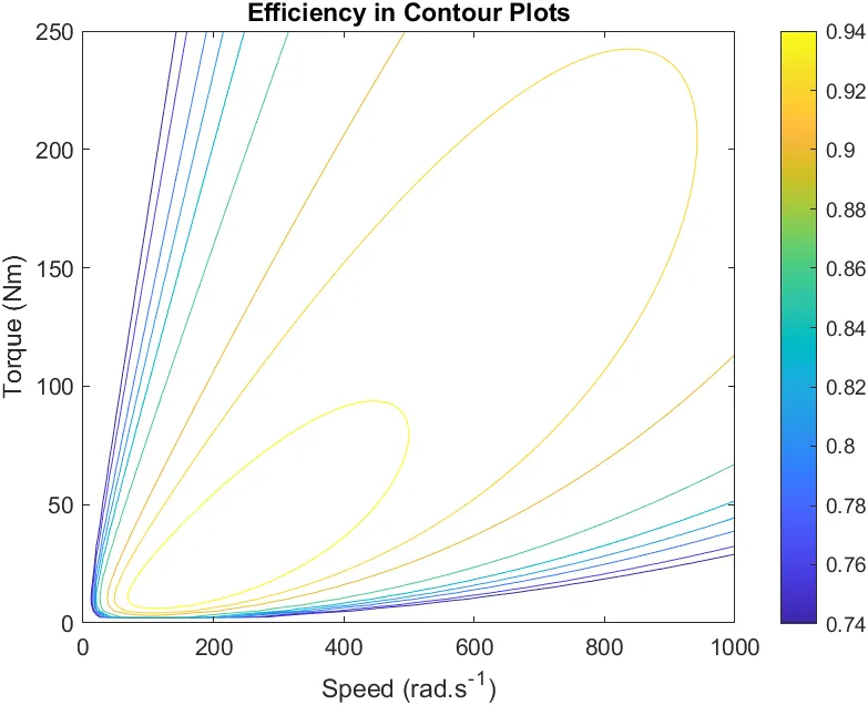
3. Make a MATLAB program which plots contour of given motor speed, torque and efficiency values. Attach the code as a .m file attach a screenshot of all the plots

Here the matlab program of efficiency contour plot has given in the following,

clear all
close all
clc

%Create Efficiency contour plots of given motor speed, torque and efficiency values

%Setup arrays for range by using linspace
x = linspace(0,1000);   %Motor speed - x axis
y = linspace(0,250);    %Torque - y axis

%Motor Loss Constants
Kc = 0.2;       %For Copper Loss
Ki = 0.008;     %For Iron Loss
Kw = 0.00001;   %For Windage Loss
ConstL = 20;     %For Constant Motor Loss

%Make Mesh
[X,Y] = meshgrid(x,y);  %To create 3D array
output_power = (X.*Y);  %Power,P = Speed*Torque
B = Kc*(Y.^2);  %For Copper Loss
C = Ki*X;       %For Iron Loss
D = Kw*(X.^3);  %For Windage Loss
input_power = output_power+B+C+D+ConstL;
Z = output_power./input_power;  %Efficiency

%Set efficiencies for the contour plot
V = [0.74,0.76,0.79,0.81,0.83,0.86,0.90,0.92,0.94]; %Mapping

%Plotting
contour(X,Y,Z,V);
grid off;
xlabel('Speed (rad.s^-^1)');
ylabel('Torque (Nm)');
title('Efficiency in Contour Plots');

EXPLANATION:

• Here we have make a countour plot with the motor speed, torque and efficiency values in matlab, so first gather some data for the inputs
• Now setup arrays for range of x-axis (motor speed) and y-axis (torque) by using the linspace command
• Then make sure with the inputs of motor loss constants, usually these details are given by the motor designer
• After that make a mesh to create 3D array by uusing the meshgrid command, then calculate output power by the power formula
• And also calculate the three varient constant losses which are copper loss, iron loss and windage loss
• Then calculate the overall input power by adding the all losses and output power, these input and output power calculation helps to find the efficiency of the motor
• By these calculations set the efficiencies for the contour plot by mapping the various random efficiencies
• And finally make a contour plot with the calculated values of motor speed, torque, efficiency and set of efficiencies

PLOT GRAPH:

CONCLUSION:

• Definition of drive cycle has explained
• The calculation for the energy required for braking has learned
• The concept of braking torque and the electric and mechanical brakes are coordination were understood
• Creation of matlab program of a contour plot for plot a motor efficiency has done