Week-11 Challenge: Braking
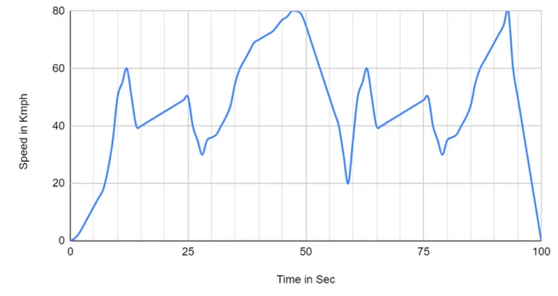
1>>Ans: Initially the drive cycle is determined in a table and plots are made using these values from the braking regions of the vehicle are taken. The plot of the drive cycle is shown below:
| Time in Sec | Speed in Kmph |
| 0 | 0 |
| 1 | 1 |
| 2 | 3 |
| 3 | 6 |
| 4 | 9 |
| 5 | 12 |
| 6 | 15 |
| 7 | 18 |
| 8 | 25 |
| 9 | 35 |
| 10 | 50 |
| 11 | 55 |
| 12 | 60 |
| 13 | 50 |
| 14 | 40 |
| 15 | 40 |
| 16 | 41 |
| 17 | 42 |
| 18 | 43 |
| 19 | 44 |
| 20 | 45 |
| 21 | 46 |
| 22 | 47 |
| 23 | 48 |
| 24 | 49 |
| 25 | 50 |
| 26 | 40 |
| 27 | 35 |
| 28 | 30 |
| 29 | 35 |
| 30 | 36 |
| 31 | 37 |
| 32 | 40 |
| 33 | 43 |
| 34 | 47 |
| 35 | 55 |
| 36 | 60 |
| 37 | 63 |
| 38 | 66 |
| 39 | 69 |
| 40 | 70 |
| 41 | 71 |
| 42 | 72 |
| 43 | 73 |
| 44 | 75 |
| 45 | 77 |
| 46 | 78 |
| 47 | 80 |
| 48 | 80 |
| 49 | 79 |
| 50 | 75 |
| 51 | 70 |
| 52 | 65 |
| 53 | 60 |
| 54 | 55 |
| 55 | 50 |
| 56 | 45 |
| 57 | 40 |
| 58 | 30 |
| 59 | 20 |
| 60 | 35 |
| 61 | 50 |
| 62 | 55 |
| 63 | 60 |
| 64 | 50 |
| 65 | 40 |
| 66 | 40 |
| 67 | 41 |
| 68 | 42 |
| 69 | 43 |
| 70 | 44 |
| 71 | 45 |
| 72 | 46 |
| 73 | 47 |
| 74 | 48 |
| 75 | 49 |
| 76 | 50 |
| 77 | 40 |
| 78 | 35 |
| 79 | 30 |
| 80 | 35 |
| 81 | 36 |
| 82 | 37 |
| 83 | 40 |
| 84 | 43 |
| 85 | 47 |
| 86 | 55 |
| 87 | 60 |
| 88 | 63 |
| 89 | 66 |
| 90 | 69 |
| 91 | 72 |
| 92 | 75 |
| 93 | 80 |
| 94 | 60 |
| 95 | 50 |
| 96 | 40 |
| 97 | 30 |
| 98 | 20 |
| 99 | 10 |
| 100 | 0 |
The figure of Drive Cycle is as follows:
Vehicle weight = 100kgs
| No of Braking | Initial Velocity (kmph) |
Final Velocity (kmph) |
Time Required (s) | Deceleration (m/s^2) | Energy Required (j) | Braking Power (W) | Braking Energy (Wh) |
| 1 | 60 | 40 | 3 | 1.85 | 277778 | 92592.6 | 25.7 |
| 2 | 50 | 30 | 3 | 1.85 | 222222 | 74074.1 | 20.6 |
| 3 | 80 | 20 | 11 | 1.52 | 833333 | 75757.6 | 21.0 |
| 4 | 60 | 40 | 3 | 1.85 | 277778 | 92592.6 | 25.7 |
| 5 | 50 | 30 | 3 | 1.85 | 222222 | 74074.1 | 20.6 |
| 6 | 80 | 0 | 7 | 3.17 | 888889 | 126984.1 | 35.3 |
Therefore the total braking energy required is 148.9 Wh
2>>Ans: This situation generally occurs when the vehicle is at high speed because the motor will be running at the constant power region in the constant power region the torque of the motor reduces and so the motor reduces and so the motor cannot develop the braking torque which is equal to the torque that occurs during low speed at the constant torque range.
The torque and speed plot of a vector control induction motor is given below:
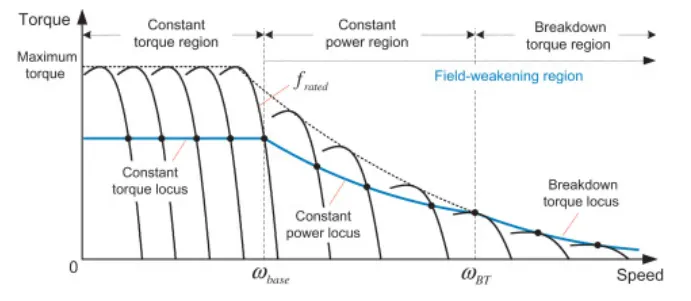
From the above characteristics curves of the motor, that is seen the torque of the motor remains high at low speeds and reduces as the speed increases. Since the electric motor cannot develop braking torque at a higher speed similar to starting.
Electrical Brake and Mechanical Brake :
Electrical Brake:
Electrical braking can be done by many methods such as
- unbalancing the input points of current to the motor
- using transistors in H bridge arrangement to reverse the motor direction in order to reduce speed
- implementing a regenerative braking system by using bi-directional power converters
- regenerative braking converts much of the energy to electrical energy which may be collected for later use
Mechanical Braking:
Mechanical brakes commonly use friction between two surfaces pressed together to convert the kinetic energy of the moving object into heat, though other methods of energy conversion may be employed the friction between the surfaces is performed using pressurized air or pressurized oil which are commonly known as sir brake and hydraulic brake respectively.
Coordination of electrical and mechanical braking in EVs:
Two types of brake control strategies are used to organize the electrical brake and mechanical brake they are as follows :
- Series control strategy
- Parallel control strategy
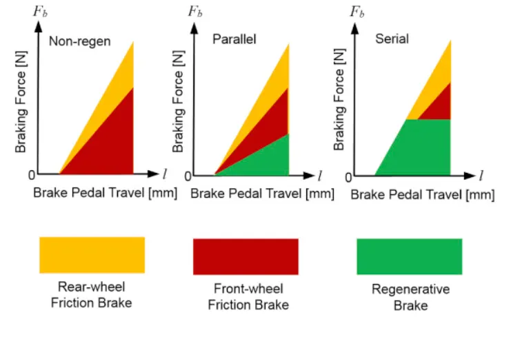
The comparison of the control strategies is shown in the below figure:
In the figure, it is seen that according to the amount of brake pedal travel of the vehicle. The mechanical brakes and regenerative brakes are employed.
Parallel Control Strategy :
When the brake is applied according to the brake pedal travel the front wheel friction brake the rear wheel friction brakes and the regenerative brakes are employed simultaneously. The higher the travel of the brake pedal the higher the amount of braking will be done. The braking energy is distributed in the following practice:
Rear Wheel Friction Brake ------> Front Wheel Friction Brake ----------> Regenerative Brake.
Series Control Strategy: When the brake is applied according to the brake pedal travel the front wheel friction brake the rear wheel friction brakes and the regenerative brakes are applied one after another. As the braking requirement increases the frictional brakes are used subsequently. for the low speed of the vehicle, regenerative braking is used but it is maybe limited according to the SOC of the battery. As the speed of the vehicle increases the rear wheel frictional brake will be employed if the braking requirement is not done then the front wheel frictional brake is also used. The coordination of the series control braking can be done with the choice of the comfort of braking.
Electric Driven Intelligent Brake: EDIB is a brake control strategy which is developed by NISSAN. It is the type of parallel braking which can be seen in the below image:
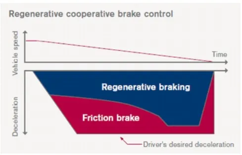
The above image shows that the frictional brake and the regenerative brake are used simultaneously at higher speeds of the vehicle. At low speed the torque of the motor is high and so the regenerative brake has a higher braking part than the frictional brakes.
Working of EDIB:
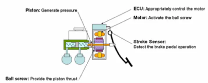
when the driver steps on the brake pedal, the stroke sensor detects the operation of the brake. That report is communicated to the ECU and controls the motor. The motor engages the piston through the ball screw and increases the friction brakes pressure through optimum control of the friction brakes hydraulics pressure the energy regeneration results is maximized.
3>> Ans: The Matlab programme for plotting control plot of motor speed, torque and efficiency is as follows:
clear all;
close all;
clc;
w=linspace(0,100);
T=linspace(0,300);
kc=0.18;
ki=0.006;
kw=0.000015;
[X,Y]=meshgrid(w,t)
copper_loss=(Y.^2)*kc;
iron_loss=X*ki;
windage_loss=(X.^3)*kw;
k=20;
output_power=x.*y;
input_power=(copper_loss)+(iron_loss)+(windage_loss)+(output_power)+k;
Eff=(output_power)/(input_power);
n=linspace(0.7,0.95,10);
contourf(X,Y,Eff,n);
title('Speed Torque Characterstics')
xlabel('Speed rad/s')
ylabel('Torque N-m')
The graph for the above Matlab programme is as follows:
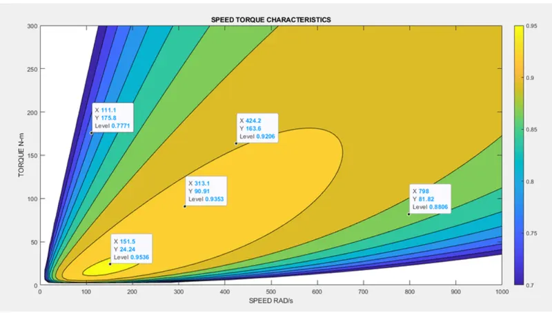
Thus from the above output graph, we could see that only at a particular speed and torque the efficiency is maximum at 95% where speed x=151rad/s @24N-m Torque.
As the speed increases the efficiency of the motor will be reduced.