Week-11 Challenge: Braking
Aim: Study the regenerative braking and energy required during braking for the electrical vehicle and plot the contour graph for the given motor speed, torque, and efficiency by using the Matlab code.
Objective:
- Study the energy required for braking during the driving cycle.
- Study about control strategies during braking conditions.
- Plot the contours of the motor speed, torque, and efficiency by using Matlab code.
Theory:
1.For a defined driving cycle, calculate the energy required for braking.
Drive cycle: Drive cycle consists of real-time data of the speed of the vehicle w.r.t. time.
There are different types of the driving cycle available for the real-time simulation of the electric vehicle, which is plotted based on the real situations
The driving cycle is used in electric vehicles for various purposes such as for calculating the range of the EV, checking the capacity of the battery for different acceleration and hill-climbing testing in simulation, also t check the SOC of the battery.
For calculating the brake energy we are using Worldwide harmonized Light vehicles Test Cycles(WLTC). I this driving cycle we have three types which are class1, class 2, and class 3.
This WLTC are classified on the basis of the power to weight ratio of the vehicle as follows:
`PW_r = (P_max)/m_v`
- Class 1 = low power vehicles with PWr <= 22
- Class 2 = vehicles with 22 < PWr <= 34
- Class 3 = high-power vehicles with PWr > 34
For our simulation we are considering the class 3 WLTC driving cycle and we have taken all speed points w.r.t time in excel sheet and the link of the excel sheet is as follows:
WLTC class 3 drive cycle Excel sheet
We know that the total energy of the vehicle is kinetic energy so for easy simplification we are considering that half of the kinetic energy is braking which is given as follows:
Braking Energy: `1/2*M_v*(V_f^2-V_i^2)`...............................................(1)
whereas,
`M_v`= Weight of the vehicle in Kg
`V_f` = Final velocity of the vehicle(m/s)
`V_i` = Initial velocity of the vehicle(m/s)
Matlab Code for calculation of braking energy for WLTC class 3 cycle:
clear all
close all
clc
% MATLAB program for calculating braking energy for the given driving cycle
%Importing Excel sheet data of WLDC cycle in the matlab
D = xlsread('WLTC_cycle.xlsx');
% mass of the vehicle in Kg
m = 2000;
%importing 1st column from drive cycle which is time(s)
T = D(:,1);
%Importing 2nd column from drive cycle which is speed(Km/h)
v = D(:,2);
%converting speed from Km/h to m/s
V = v*(5/18);
%Total time of the cycle
t = 1801; % sec
% To plot graph we have to make the vector of the both variables.
Braking_energy = zeros(1,t);
Deceleration = zeros(1,t);
TOTAL_ENERGY = zeros(1,t);
for i= 1:(length(V)-1)
    if V(i+1)<V(i)
        Deceleration(i)= V(i+1)-V(i);
        % As time difference is 1 constant through out the cycle
        Braking_energy(i) = 0.5*m*((V(i+1))^2-(V(i))^2)/3600000;
    end
    TOTAL_ENERGY(i) = 0.5*m*((V(i+1))^2-(V(i))^2)/3600000; %KWh
end
%Total energy in KWh for WLTC class 3 drive cycle
Total_energy = sum(abs(TOTAL_ENERGY));
fprintf('Total energy generated by WLTC class 3 drive cycle is= %1.2f KWh \n',Total_energy );
% Braking energy in KWh for WLTC class 3 drive cycle
T_B_E = -1*sum(Braking_energy);
fprintf('Total braking energy generated by WLTC class 3 drive cycle is = %4.4f KWh', T_B_E);
% Plotting the WLTC class 3 drive cycle by using given data
subplot(3,1,1)
plot(T,v,'color','r','linewidth',1.5)
xlabel('Time(s)')
ylabel('Speed(km/h)')
title('WLTC Class 3 cycle')
grid on
%plotting the braking energy for given drive cycle
subplot(3,1,3)
plot(T,-Braking_energy,'color','g','linewidth',1.5)
xlabel('Time(s)')
ylabel('Braking Energy(KWh)')
title('Braking Energy graph')
grid on
% plotting the deceleration done for given drive cycle
subplot(3,1,2)
plot(T,Deceleration,'color','y','linewidth',1.5)
xlabel('Time(s)')
ylabel('Deceleration(m/s^2)')
title('Deceleration graph')
grid on
figure(2)
plot(T,TOTAL_ENERGY,T,Braking_energy)
legend('TOTAL_ENERGY','Braking_energy')
Explanation of the Matlab program:
1.First step is to call the excel sheet data in MatLab by using 'xlsread(filename)'.
2.Now we define the first column as a time and the second column as speed in Kmph. as our speed is in the Kmph so we convert that speed into m/s by multiplying the speed column by 5/18 factor.
3.We define the mass of the vehicle as 200Kg and drive cycle time is 1801, we have added plus one to the drive cycle to calculate the deceleration at the end.
4.In the 'for loop' to the range of first value to the end-1 values of the speed we calculate the deceleration for 'if condition' which is the final speed should be less than the initial speed. for deceleration, we take the difference between two consecutive speeds. and for brake energy, we use equation 1 within this 'if condition'. we have divided the braking energy equation with 3600000 to convert it from J to KWh.
5.Now we end the for loop and to calculate the total braking energy we do the sum of all the braking energy.
6.Now we plot the graphs for driving cycle, braking energy, and deceleration w.r.t. time by using plot and subplot command in Matlab.
Output:
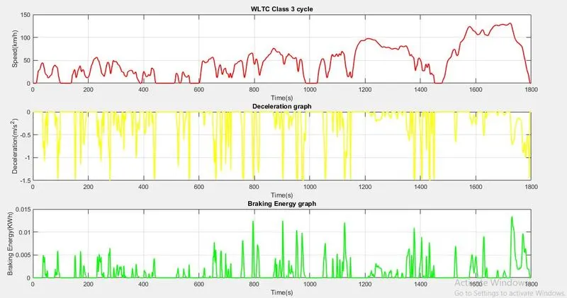
1. Graph of the WLTC class 3, braking energy, and deceleration w.r.t. time is as follows:
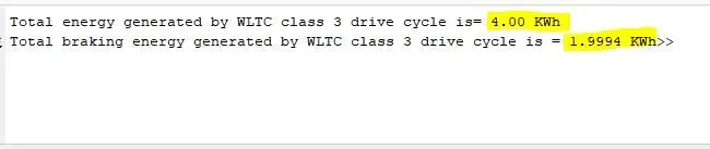
2.Total energy and braking energy in KWh:
Conclusion:
So from the above result, we can say that braking energy produced due to brake is nearly half of the total energy, so if we use regenerative braking it can increase the range of the EV oR HEV
2.Why electric motor can’t develop braking torque at a high speed similar to starting? How electric and mechanical brakes are coordinated?
Let us see the behavior of the motor in the torque vs speed graph, as shown below,
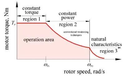
As we can see that for the zero speed the torque is maximum and it is constant up to the rated speed so this region where speed is below rated speed or critical speed is called the constant torque region, so here we have maximum torque which is for lower speed, After constant torque region, we have constant power region where we keep the power constant by decreasing the torque and increasing the speed by doing field weakening technique. so at a higher speed, we have less torque produced. Also at lower
Types of electrical and mechanical brake co-ordination:
As we know that while braking the vehicle we have to stop the rear wheel first and then we have to stop the front wheel in order to achieve the stable braking of the vehicle.
1. Series Brake: In series brake, we apply mechanical and electrical brakes one after another, or we apply only one type of braking either mechanical or electrical. In this, we have two types which are as follows,
a.)series braking system with an optimal feel: The series braking system with an optimal feel consists of a braking controller that controls the braking forces on the front and rear wheels. The purpose of this strategy is to minimize the stopping distance and optimize the driver’s feel. The shortest braking distance and good braking feel require the braking forces on the front and rear wheels to follow the ideal braking force distribution.
b.)series braking system with optimal energy recovery The principle of a series braking system with optimal energy recovery is to recover the braking energy as much as possible in the condition of meeting the total braking force demanded given deceleration.
2.Parallel Brake: In this braking strategies we apply both electrical and mechanical brakes in parallel and simultaneously by considering that the rear wheel should be the first lock and after that the front wheel should lock to get stable braking.
3.Electrical driven intelligent brake(EDIB):
This control strategy is developed by the Nissan company in 2006 under Nissan green program 2010. because conventional cooperative regenerative braking systems have not been able to fully recover kinetic energy during deceleration owing to the difficulty of reconciling energy regeneration with braking performance and vehicle behavior.
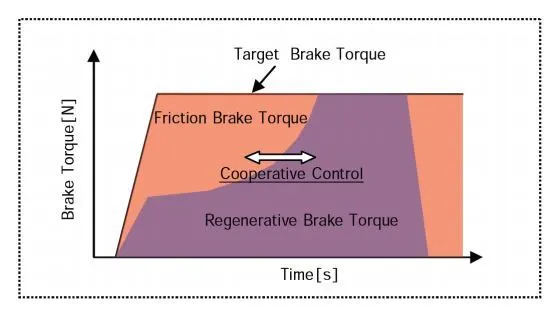
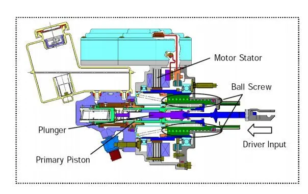
This is the diagram of the EDIB strategies in which at starting where speed is more and the more resistance torque is required their it uses mechanical braking so as time goes on and speed getting decreasing then electrical braking is applied simultaneously and at target brake torque we have maximum electrical braking torque and less mechanical braking as shown in the above diagram.
Features of the EDIB:
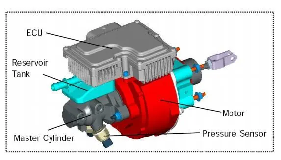
1.It incorporates a mechanism for directly converting the rotational motion of an electric motor integrated into the brake unit for use as the booster source instead of using the engine manifold vacuum as conventional brake systems do.
2.It reconciles cooperative energy regeneration with braking performance matching the vehicle characteristics by the brake unit built without a stroke simulator.
Internal and external schematic diagram of the EDIB:
3.Make a MATLAB program which plots the contour of given motor speed, torque, and efficiency values. Attach the code as a .m file attach a screenshot of all the plots.
clear all
close all
clc
% Motor data from the specification
Peak_torque=[0 330;2620 324;2840 319;2950 311;3110 296;
                3290 279;3490 262;3690 243;3910 225;
                4130 208;4440 187;4650 175;5020 157;
                5310 145;5600 134;5980 122;6360 112;
                6960 99;7440 90;8040 80;8750 73;
                9180 68;9650 63;10200 59;10600 56]; % [rpm Nm]
continuos_torque=[0 271;873 270;1840 265;2490 260;2960 256;
                3130 247;3380 231;3560 220;3800 205;
                4070 190;4380 175;4580 165;4820 155;
                5090 144;5470 131;5840 121;6290 109;
                6840 97;7360 87;7800 80;8400 73;
                8960 67;9870 58;10600 51]; %[rpm Nm]
N=linspace(0,10600,60); % [rpm]
Tq=linspace(0,350, 60); % [Nm]
N_p=Peak_torque(:,1); % [rpm]
Tq_p=Peak_torque(:,2); % [Nm]
N_c=continuos_torque(:,1); % [rpm]
Tq_c=continuos_torque(:,2); % [Nm]
kc=0.1; % [W/Nm^2]
ki=0.0; % [W/(rad/s)]
kw=1.0e-5; % [W/(rad/s)^3]
C=500; % [W]
effMin=0.1;
omega=N*pi/30; % [rad/s]
for i=1:length(omega)
    for j=1:length(Tq)
        P_out(i,j)=(omega(i)*Tq(j)); % [W]
        P_loss(i,j)=kc*Tq(j)^2+ki*omega(i)+kw*omega(i)^3+C; % [W]
    end
end
eff=max(effMin,P_out./(P_out+P_loss))*100;
V=[10,20,30,40,50,60,70,85,90,91,92,93,94,95,96,97,98,99];
box off
contourf(N,Tq,eff,V,'showtext','on');
colorbar
hold on
plot(N_p,Tq_p,'b','LineWidth', 2);
hold on
plot(N_c,Tq_c,'r','LineWidth', 3);
text(4580,165,'\leftarrow continuous condition','fontsize',15,'color','r')
text(3690,243,'\leftarrow peak condition','fontsize',15,'color','r')
grid on
xlabel('Motor Speed [rpm]');
ylabel('Motor Torque [Nm] & Motor efficiency [%]');
title('Motor efficiency');
Explanation of the MATLAB program:
1.The first step is to get the specification of the motor which consists of speed and torque data for continuous condition and peak condition and defining them to plot the speed-torque graph for the range.
2.We know the boundary(maximum) values of the torque and speed so we divide them into equal parts by using linspace command.
3.We have defined the values of the speed and torque for the continuous and peak condition now we call this variable and define them for the next further calculation.
4.Now we define the constants which are Kc, Ki, Kw which are associated with copper loss, iron loss, and windage loss.
5.Next we define the minimum efficiency of the motor up to which we have to plot the efficiency graph and we convert the defined speed which is in rpm to the rad/sec.
6.Now we calculate the output power for the range of the torque and speed(rad/sec), and after that, we calculate the total losses. which is the addition of the copper, iron, and windage losses in the for a loop.
7.Next to get the maximum value between the defined value and the calculated value we use the max command which gives the maximum value between them.
8.Now we define the contour line values i.e for this efficiency we get contour lines on the graph. Next to plot the contour graph we define speed on the x-axis, torque on the y-axis, efficiency on the Z-axis, and the contour lines of the efficiency.
9.Last step we plot the torque-speed graph for the peak and continuous conditions of the motor.
Output:
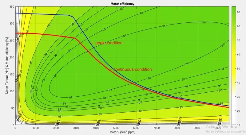
Conclusion: So from the above graph, we can get the range of the torque and speed values for which we get the maximum efficiency, we can also get the point for which efficiency is maximum with is the torque-speed graph of the motor.