Week-11 Challenge: Braking

1.Braking power:

The braking power is calculated with the UDDS drive cycle.The drive cycle contains data with 1370 time period.

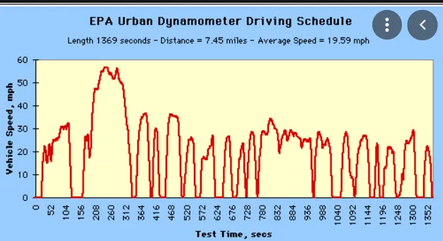
The drive cycle value is uploaded into the mathlab as a excel file.

The braking power is calculated from the formula,

p=1/2*mass*(Vi^2-Vf^2)

Vi=initial velocity

Vf=final velocity

%input
m=1500+0.05*(1500);
g=9.8;
time_period=1370;
num=xlsread('UDDS.xlsx');
time=num(1:time_period,1);
v=num(1:time_period,2);
instataneous_braking_energy=zeros(1,time_period);
%loop
for i=1:(length(v)-1)
    if v(i)>v(i+1)
       instataneous_braking_energy(i)=0.5*m*0.001*(((v(i)*0.447)^2-(v(i+1)*0.447)^2/3600));
    end
end
plot(time,instataneous_braking_energy,'m')
xlabel('Time(s)')
ylabel('Braking energy')
title('Braking energy values for UDDS drive cycle')
fprintf('The total braking energy required for UDDS drive cycle is %3f kwh',sum(instataneous_braking_energy))

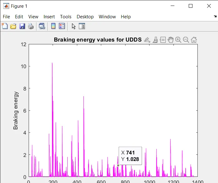
The above code is used to obtain the braking power of the vechicle

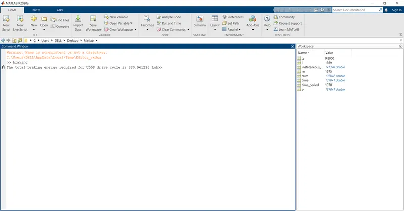
The total amount of braking power needed for the vechicle in the UDDS drive cycle is about330kwh.

2.Electric braking-Mechanical braking:

The motor characteristics is not same during the forward motoring and the braking period.

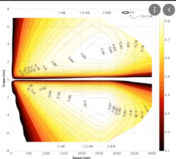
During the acceleration ofmotoring operation the speed of the motor is low so the torque produced is large but during the deceleration already the motor is in top speed which may be beyond the synchronous speed so the torque produced is of low value.

Coordination between electric braking and mechanical braking:

Two basic questions arise while considering regenerative braking in EVs and HEVs:
i. How to distribute the total braking forces required between the regenerative brake and the mechanical friction brake so as to recover the kinetic energy of the vehicle as much as possible.
ii. The other is how to distribute the total braking forces on the front and rear axles so as to achieve a steady-state braking.
Basically, there are three different brake control strategies: series braking with optimal braking feel; series braking with optimal energy recovery; and parallel braking.

Series braking with optimal braking:

The control objective is to minimize the stopping distance and optimize the driver’s feel.When the commanded deceleration (represented by the braking pedal position) is less than 0.2g, only the regenerative braking on the front wheels is applied, which emulates the engine retarding function in conventional vehicles. When the commanded deceleration is greater than 0.2g , the braking forces on the front and rear wheels follow the ideal braking forces

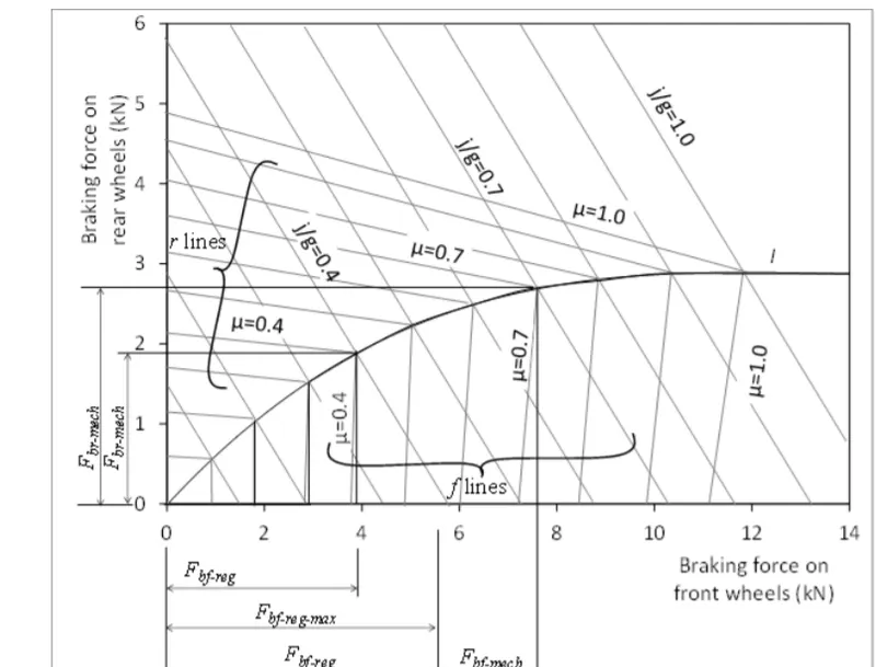
It should be noted that the maximum regenerative braking force produced by an electric motor is closely related to the electric motor’s speed. At low speed (lower than its base speed), the maximum torque is constant. However, at high speed (higher than its base speed), the maximum torque decreases hyperbolically with its speed. Therefore, the mechanical brake torque at a given vehicle deceleration varies with vehicle speed.

Series braking with optimal energy recovery:

The principle of the series braking system with optimal energy recovery is to recover the braking energy as much as possible in the condition of meeting the total braking force demanded for the given deceleration.When the vehicle is braked with an acceleration rate of j /g<u, the braking forces on the front and rear wheels can be varied in a certain range, as long as the Fbf +Fbr=Mvj is satisfied.

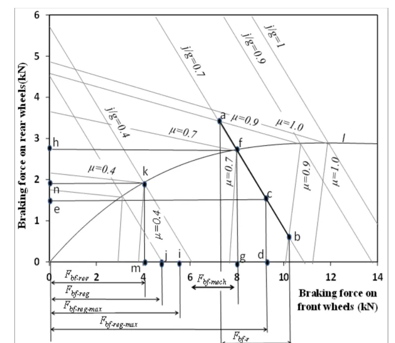
It should be noted that the series brake with both optimal feel and energy recovery needed active control of both electric regenerative braking and mechanical braking forces on the front and rear wheels. At present, such a braking system is under research and development.

Parallel braking:

The parallel brake system includes both an electrical (regenerative) brake and a mechanical brake, which produce braking forces is parallel and simultaneously The parallel brake system has a conventional mechanical brake which has a fixed ratio of braking force distribution on the front and rear wheels. Regenerative braking adds
additional braking force to the front wheels, resulting in the total braking force distribution curve.

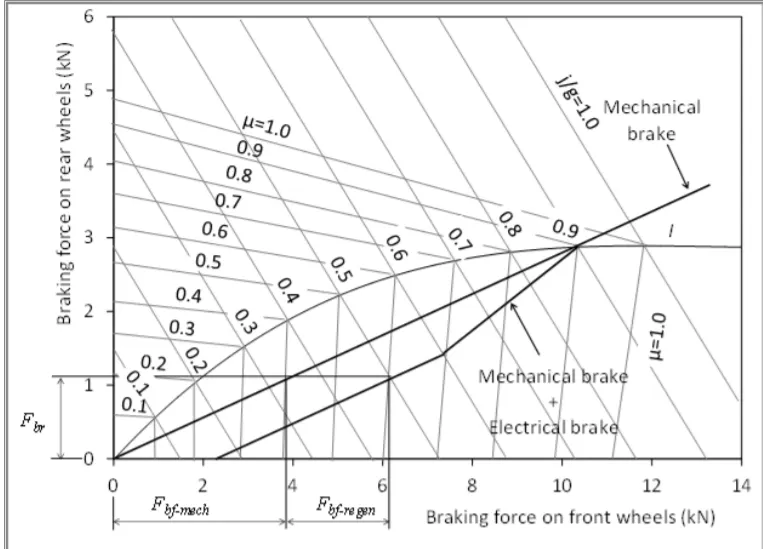
The pressure signal is regulated and sent to the electric motor controller to control the electric motor to produce the demanded braking torque. Compared with the series braking of both optimal feel and energy recovery, the parallel braking system has a much simpler construction and control system. However, the driver’s feeling, and amount of energy recovered are compromised.

3.Frequency contour:

The mathlab code for obtaining the contour is shown below,

speed=linspace(1,1000);
torque=linspace(1,250);
kc=0.2;  %copper loss constant
ki=0.008;   %iron loss constant
kw=0.00001;    %windage loss constant
con=20;      %constant loss
[X,Y]=meshgrid(speed,torque);
Output_power=(X.*Y);
Cu_loss=(Y.^2)*kc;
Ir_loss=X.*ki;
Wi_loss=(X.^3)*kw;
Input_power=Output_power+Cu_loss+Ir_loss+Wi_loss+con;
Efficiency=Output_power./Input_power;
V=[0.7,0.75,0.8,0.85,0.90,0.91,0.92,0.93];
box off
grid off
contourf(X,Y,Efficiency,V);
colorbar
xlabel('Speed(rpm)')
ylabel('Torque(Nm)')
zlabel('Efficiency')
title('Speed-Torque efficiency')

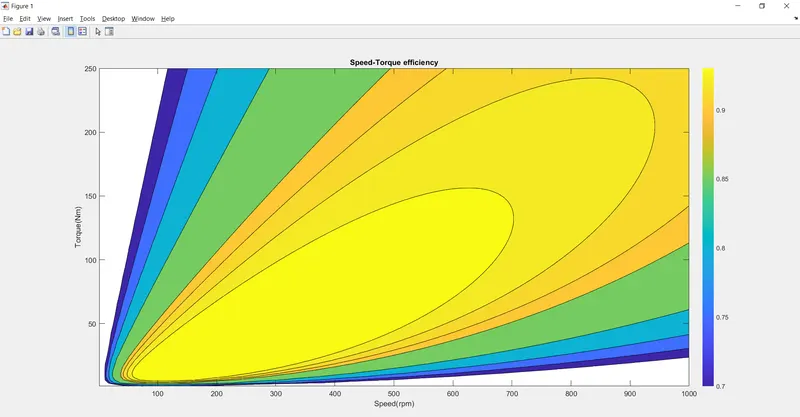
The result obtained is the contour of differant frequency for the speed torque relationship,