Week-11 Challenge: Braking

1. For a defined driving cycle, calculate the energy required for braking.

We will start by defining the drive cycle for 25 seconds, once the drive cycle is defined

we will start by identifing breaking nodes in the drive cycle

we have prepared excel finne in which we have entered all the data and braking mode data is noted in the separate table

using formula

`KE = 1/2 m v^2`

we considered vehical mass as 500kg for this example

and v will be in m/s

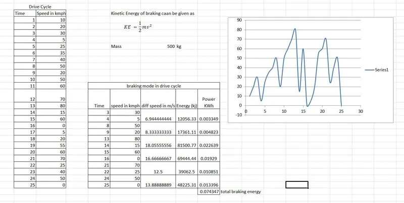
the total braking energy is 0.0743 kwh

2. Why electric motor can’t develop braking torque at high speed similar to starting? How electric and mechanical brakes are coordinated?

• As in motor torque speed characteristics the motoring (1 quadrant) and generating (3^rd quadrant ) are mirror image, in 1 st quadrant with the motor can develop high torque with less speed same, in 3^rd quadrant at lover speed the torque value at lower speed will be much negative than at higher speed so the motor cannot develop sufficient breaking power at lower speed, refere below image

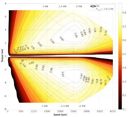
• The regenerative braking torque cannot be made large enough to provide all the required braking torque of the vehicle as it might lead to the deterioration in stability of the vehicle. Also as compared to the torque values of acceleration torque of motor is much higher than decceleration torque.
• At high speed, the motor might be in its constant power region which causes less values of torques produced and this limits the amount of braking torque that is used for regeneration. Hence the peak vlaue of accleration torque and braking torque are not equal.

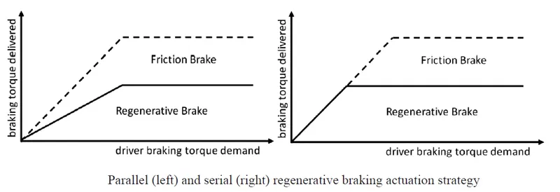
In general, EVs are equipped with the regenerative-hydraulic hybrid braking system. Whenever the regenerative braking torque is insufficient to offer the same deceleration rate as available in conventional vehicles, the hydraulic braking torque is applied.

In two methos we can cordinate the mechanical and electrical braking, seriea and parallel method

3 Make a MATLAB program which plots contour of given motor speed, torque and efficiency values. Attach the code as a .m file attach a screenshot of all the plots.

clear all
close all
clc
omega = linspace(0,1000);
torque= linspace(0,250);

%Motor Loss constants
%for copper loss
k_c = 0.2;
%for iron loss
k_i = 0.008; 
%for winding loss
k_w = 0.00001; 
% for conduction  loss
cl = 20;

% Making 2d matrix
[T,W] = meshgrid(omega,torque);

%  Output power = torque*Speed
Out_power = (T.*W);

% Copper Loss
b = (W.^2)*k_c;

% Winding Loss
c = (T.^3)*k_w;

% Iron Loss
d = T*k_i;

% Therefore for Input Power
In_power = Out_power +b +c +d +cl;

% Efficiency
E= Out_power./In_power;

%Efiiciency levels for contour
e=[0.70,0.75,0.80,0.82,0.87,0.89,0.90,0.92];

%Creating Contour
contourf(T,W,E,e);
xlabel('Speed');
ylabel('Torque');
title('Contour for Motor speed,Torque and Efficiencies')

Plot:

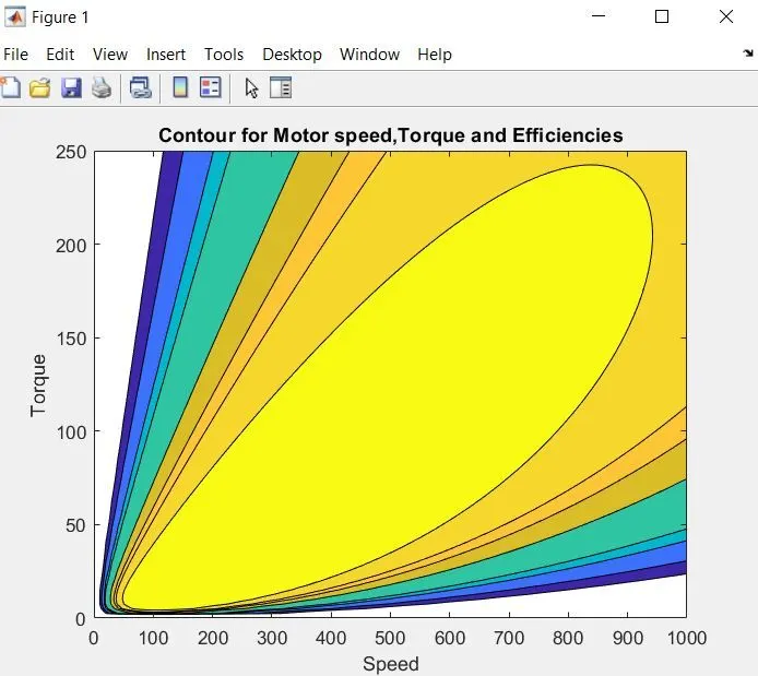
The contour plot for a motor with defined constants are plotted in the defined Speed Vs Torque Region based on efficiency. It can be seen that for increasing speed and torque, the efficiency of the motor gradually decreases. The level of efficiency is depicted using colorbar.