Week-11 Challenge: Braking

1.

Values given for the model are:

kerb weight(kg) = 656

payload(kg) = 136

Now Braking power(kW) = (m*V^2)/(2*t) [where m = 656+136]

Braking energy(kJ) = (m*V^2)/(2)

Required Braking energy(0-20sec) = 2334.514J

Required Braking energy(20-40sec) = 1888.28J

Required Braking energy(40-85sec) = 2037.904J

Required Brake energy for my entire driving cycle (0-85sec) = 6.260kJ

Required Brake power for my entire driving cycle (0-85sec) = 0.0736kW.

The driving cycle for above energy results is attached in the below excel sheet.

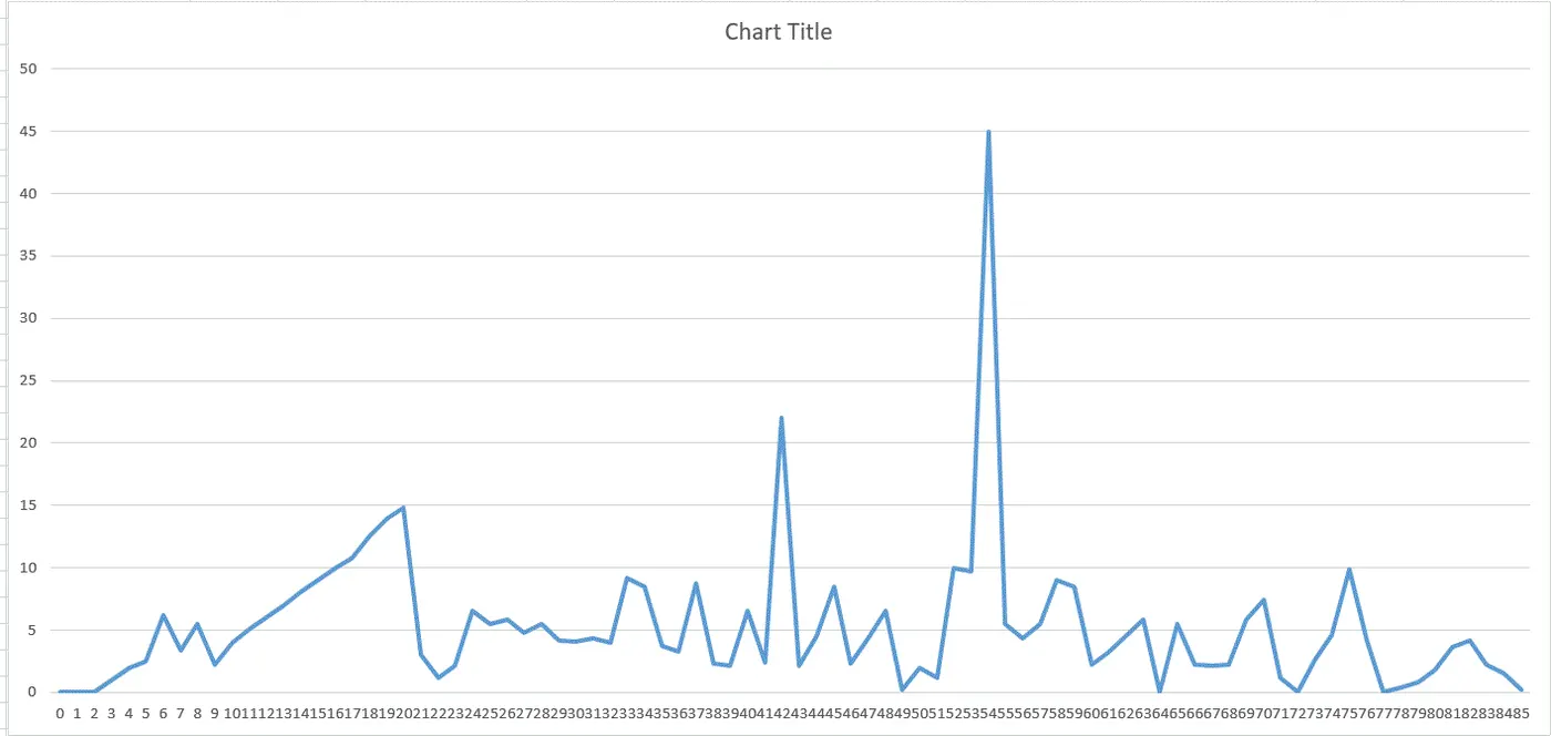
The above figure is the driving cycle output for the data we initialized.

2.

Usually during the running of an electric vehicle the energy produced is distributed to many components for the operation, among them braking is an operation that needs energy.

Here if we consider 100% of energy (from battery) then it will be distributed according to the path you are driving.

At starting some part of energy(100%) is distributed to a 'standstill and engine losses' etc., so there will be much scope for consuming energy to produce torque for braking at the starting. Whereas during high speed the 'engine losses' are increased and later much energy is distributed to 'Aerodynamic & Rolling' and less energy is available for braking.

Electrical and mechanical brakes are coordinated by control strategies namely series & parallel:

Series: In this strategy, the brakes are applied simultaneously one after the other i.e., regenerative and mechanical brake system.

Parallel: In this strategy, the brakes are applied parallelly at a time i.e., regenerative and mechanical brake system.

For this brake operation, we have EDIB(Electronic Driven Intelligent Braking) that works with the help of ECE(engine control unit)-controlled motor and ball screw arrangement which decreases the main motor burden for applying torque utilized for the brake system.

3.

The MatLab code which plots the contour of given motor speed, torque, and efficiency values is compiled and plots are obtained.

x = linspace(1,1000); % for torque

y = linspace(1,300); % for speed

Kc = 0.3; % copper loss constant

Ki = 0.006; % iron loss constant

Kw = 0.0002; %windage loss constant

Con = 15; %constant losses;

[X,Y] = meshgrid(x,y);

outputpower = (X.*Y);

B = (Y.^2)*Kc;

C = X*Ki;

D = (X.^3)*Kw;

inputpower = outputpower +B+C+D+Con;

E = outputpower./inputpower;

V = [0.65,0.73,0.78,0.83,0.85,0.90,0.925,0.936];

box off

grid off

contour(X,Y,E,V,'showtext','on')

xlabel('speed in rad/sec');

ylabel('Torque in N/m');

hold on

v = [8000,10000]; % plot between these values

contour(X,Y,outputpower,v)

end

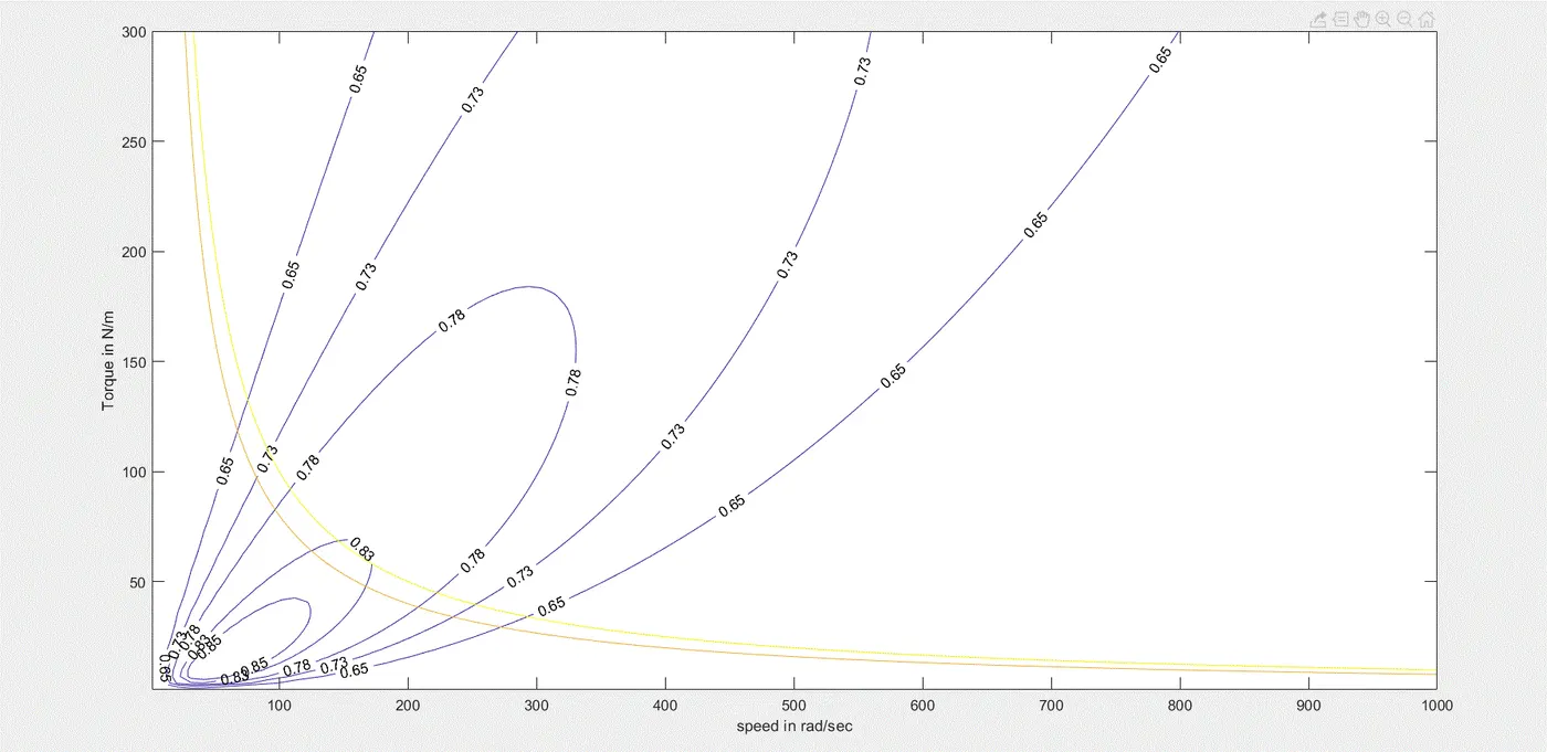
The output obtained above shows the contour where the inner circle shows the highest peak in efficiency and operation parameter whereas the yellow curves shows the plots of 8000 & 10000 kW power.