Braking in electric vehicles

AIM:

1. To calculate the energy required for braking for a defined driving cycle.
2. To understand why electric motor can’t develop braking torque at high speed similar to starting and how electric and mechanical brakes are coordinated.
3. To plot contour of given motor speed, torque and efficiency values using a MATLAB program.

SOLUTION:

1. To calculate the energy required for braking for a defined driving cycle.

In order to calculate the braking energy, the following formula is used:

Braking energy = ½(mV²)

where, m = mass considering the inertia effect

V = V_final - V_initial (velocity difference for the deceleration process)

In order to calculate the total braking energy, it is necessary to consider the deceleration over the entire cycle.

The braking energy for the ftp75 driving cycle is calculated using the following steps.

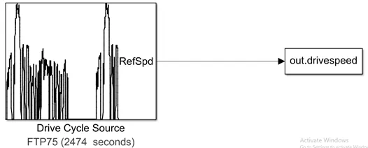
1.The Simulink ‘Drive Cycle Source’ block is used to get the drive cycle data. This data is then exported to the base workspace by using the to workspace block.

2.The following script is written to get the kinetic energy required.

Braking energy = ½(m(Vfinal - Vinitial)²

Braking energy over entire cycle = ½(m(SUM(Vfinal - Vinitial)²))

Here, Sum indicates the addition of velocity differences for various deceleration cycles over the entire cycle. The MATLAB script shows a function written in order to calculate the kinetic energy. The functions takes the velocity (m/s) array and the mass(kg) of the vehicle and returns the braking kinetic energy required by the vehicle in kilo Joules.

%function to calculate the braking energy required
%x is the velocities(m/s) array & m is the mass of the vehicle
 
function KE = brakingEnergy(x , m)
sum=0;
i=1;
len= length(x);
 
while (i < (length(x)-1))                            
    if (x(i+1) < x(i))                                %Vfinal
        v2 = x(i);
        
        while(x(i+1) <= x(i)) && (i<(length(x)-1))
            i = i+1;
        end
        
        v1 = x(i);                                     %Vinitial 
        diff = (v2-v1)^2;                              %(Vfinal - Vinitial)^2 
        sum = sum + diff;                              %Sum of all (Vfinal - Vinitial)^2 
    else
        i = i+1;
    end
end
fprintf('No. of seconds in drive cycle are %d.n', len);
KE = (0.5*m*sum)/1000;                                 %Kinetic Energy in kilo Joules 
fprintf('KE is %d KJ. n', KE);                        
end

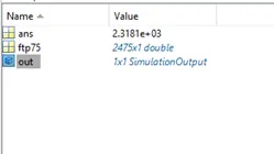
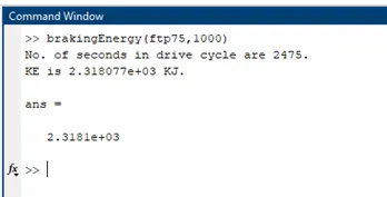
The kinetic energy required for braking is calculated for the ftp75 Drive Cycle and it is 2318 kJ.

2. To understand why electric motor can’t develop braking torque at high speed similar to starting and how electric and mechanical brakes are coordinated.

If the motor is being used as a generator, it is restricted by the same power limits as to when it is acting as a motor because vehicles typically can brake much harder with conventional, friction-based brakes. Peak torque during acceleration and deceleration are not equal. Hence electric motor can’t develop braking torque at high speed similar to starting. It is virtually impossible and actually impractical to recover all braking energy at high speed or high deceleration rates. Braking power is not only limited by the motor’s power rating, but also by the charging power limit of the battery pack. These limits depend upon the chemical composition (battery type) and changes with temperature. This makes analyzing the braking power capability difficult, as a vehicle may be able to regeneratvely brake at full-power for a short period of time but as the temperature of the battery pack rises, the braking power will quickly fall. The exact amount of energy and the rate of energy that can be recovered is dependent on the available motor, battery types and the driving scenario. A two-wheel-brakes are used, the negative torque applied result in uneven distribution of the braking energy between the wheels and further wear of the tires.

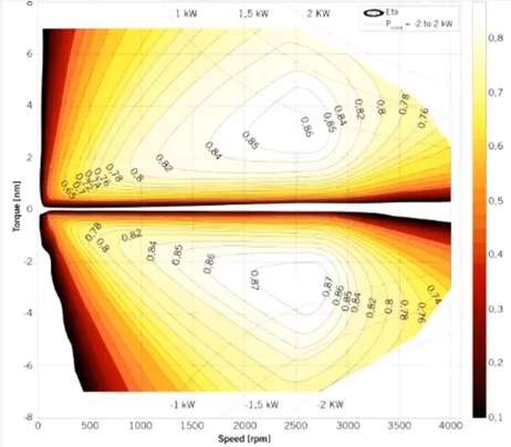
At high speeds (higher than base), the maximum torque decreases hyperbolically with its speed as indicated in the below figure. If the vehicle speed is higher, then that point lies in the constant power region of the characteristics. Here, the peak torque will be high(7N-m) whereas when the vehicle has to decelerate, the torque developed has to be negative. For the same speed, if we observe in the 4^th quadrant, the motor torque corresponding to that speed will be lower than the peak torque (which is 7N-m during starting). Hence electric motor can’t develop braking torque at high speed similar to starting.

Electric and mechanical brakes are coordinated taking into consideration the points discussed above. The different control strategies used are series braking and parallel braking.

Series braking throws in the frictional and mechanical brakes one after the other and in parallel braking, both brakes are applied at the same time considering the SOC of the Battery and other vehicle parameters.

3. To plot contour of given motor speed, torque and efficiency values using a MATLAB program.

In order to plot the speed, torque and efficiency plot,

Separate variables have been taken into consideration, like for speed X, for torque Y.

Efficiency is the ratio of output to input while calculating the input, the losses also need to take into consideration.

The losses are iron losses, copper losses, windage losses.

Copper losses = I^2.R = Kc.T^2, where Kc is the resistance of brushes coil.

Iron losses = Ki.w, this varies with speed.

As at various speed, we have different values of back emf and that will affect these losses.

Windage losses = Kw.W^3, depends on the size and shape of the motor. - Constant losses c.

Total losses = Kc.T^2 + Ki.w + Kw.W^3 + c

Variable V is efficiency points we are giving.

% Plotting efficiency contours for electric motors.
    % Arrays for range.
x=linspace(1,180);                      % speed, omega, N.B. rad/s NOT rpm
y=linspace(1,40);                       % 0 to 40 N.m
% Allocate motor loss constants.
kc=1.5;                                 % Copper loss constant
ki=0.1;                                 % Iron loss constant
kw=0.00001;                             % Windage loss constant
ConL=20;                                % Constant motor losses
% Now make mesh
[X,Y]=meshgrid(x,y);
Outputpower=(X.*Y);                     % Torque x speed = power
B=(Y.^2)*kc;                            % Copper losses
C=X*ki;                                 % Iron losses
D=(X.^3)*kw;                            % Windage losses
Inputpower = Outputpower + B + C + D + ConL;
Z = Outputpower./Inputpower;
% We now set the efficiencies for which a contour will be plotted.
V=[0.5,0.6,0.7,0.75,0.8,0.85,0.88];
box off
grid off
contour(X,Y,Z,V);
xlabel('Speed/rad.s^-^1'), ylabel('Torque/N.m');
hold on
% Contour of the power output
% The array Output Power has already been calculated. We draw contours at
% 3 and 5 kW.
V=[3000,5000];
contour(X,Y,Outputpower,V);

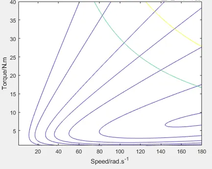
From the figure, the behaviour of torque, speed and efficiency can be observed. The innermost contour has the highest efficiency. The EV design engineer has to take care of the efficiencies.

CONCLUSION:

The challenge has the following learning outcome:

Braking energy calculations.

Coordination of electrical and mechanical braking.

Plotting of torque, speed and efficiency contours.