SYSTEM LEVEL SIMULATION OF ALL TERRAIN VEHICLE

AIM:

To perform system level simulation of Model: BAJA All-terrain vehicle (ATV) that uses CVT and analyze and interpret the results.

OBJECTIVE:

1. To study open and closed loop ATV models.
2. To understand the use of lookup tables & Dashboard blocks that enhance the performance of a Simulink Model.

MODEL ANALYSIS:

Introduction to CVT: CVTs differ from traditional automatic transmissions in that they don't have gears that provide "steps" between low- and high-speed operation. Instead, the majority of them work via a pair of variable-diameter, cone-shaped pulleys connected by a steel or composite belt.

The step-less nature of its design allows the CVT to work to keep the engine in its optimum power range, increasing efficiency and fuel mileage by delivering an infinite number of smooth transitions from low to high.

The four models under study are:

1. BAJA ATV open loop model
2. BAJA ATV open loop model and with Dashboard
3. BAJA ATV closed loop model
4. BAJA ATV closed loop model and with Dashboard

The subsystems/blocks common to all these models are the CVT, Vehicle Body, Engine and Simple Gear and scope blocks. These are explained below:

CVT: The CVT subsystem consists of the following blocks under its mask:

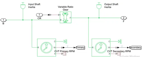
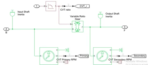
To facilitate the step-less design of the CVT, a variable ratio gear is implemented in the model and the input to this block will decide the actual gear ratio. Both the base and the follower (primary and secondary) are given inertia elements to make the model more realistic. Rotational motion sensors are connected to measure the rpm of both sides.

VEHICLE BODY: The vehicle body subsystem consists of the following blocks under its mask:

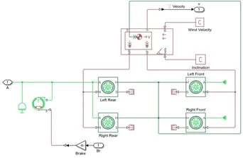
The vehicle body is defined to have a mass of 250kg mass. The four wheels are connected accordingly and rpm of the secondary of CVT and brake input are given to the subsystem. The vehicle body is given zero inclination and wind velocity. The velocity is taken to the scope by using an Outport (and goto block outside the subsystem) block.

ENGINE AND SIMPLE GEAR: To connect the CVT and the engine, a simple gear with a gear ratio of 4 is used. This transfers the torque and speed in a favorable manner from the engine to the primary shaft of the CVT.

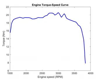
The Generic Engine block is used to model the engine of the vehicle. It is given the speed vector and torque vector by extracting the data points from the speed torque curve which is represented below

The other elements used in the models are dashboard elements and Lookup table. They are explained below.

LOOKUP TABLES (Model 3 & 4 ):

Lookup tables are used to map output/s based on input given. The output data corresponding to input is linked using a data array defined in the lookup table. The relationship between the input and output is unknown. Lookup tables improve accuracy and reduces time. Simulink can extract other data points by interpolation and extrapolation. It can be implemented by using the ‘Lookup Table’ Block.

The Lookup table used in the model gives the CVT Ratio as output for respective input vehicle speed. The vehicle speed is fed back to the CVT subsystem where the CVT ratio is calculated using the lookup table block. The visualization of the lookup table used in two of the models under study is shown below:

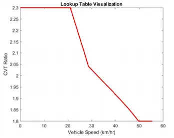
These data points were created by simulating the model (not using a lookup table) for various vehicle speeds and the CVT Ratio was recorded.

DASHBOARD ELEMENTS (Model 2 & 4):

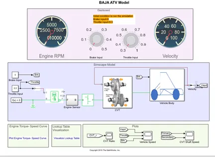
Dashboard elements allow us to give input and observe the output instantaneously during the runtime of the simulation. The two blocks used are knob and custom gauge. Using the knob, the two inputs: throttle and brake are applied, and using the Custom Gauge: RPM and velocity of the vehicle are observed.

1. BAJA ATV open loop model

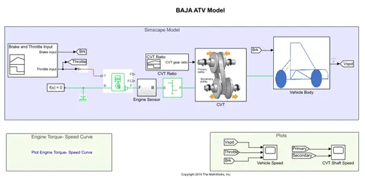
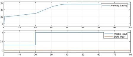
This is the ATV in its simplest form. The inputs are given by the signal builder block and CVT ratio decreases linearly from 2.3(t=4) to 1.8(t=35). Here, the brake input provided is zero for the entire time and throttle applied is 0.3 till 20secs whereas full Throttle is applied after 20secs to the engine. The initial rpm of the engine is specified to be 2100rpm. The results of the simulation are as follows

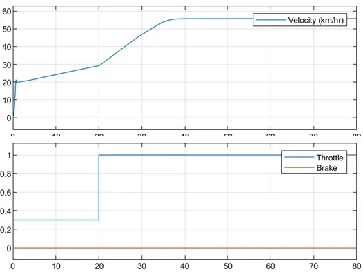
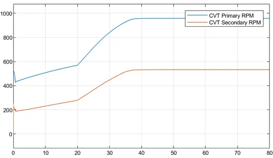
Here, there are 3 time intervals of interest. t=0 to t=4 (say T1), t=4 to t=20 (say T2), t=20 to t= 35 (say T3) and t=35 to t=80 (say T4)

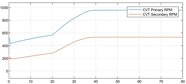
During T1, since the gear ratio and throttle are constant, there is linear variation between the primary and secondary rpm. During T2, the throttle is still constant, but now, gear ratio starts decreasing. This increases the speed of the vehicle. At t=20sec, the throttle input jumps to 1 and therefore, the speed rises at and increased rate. And continues to rise owing to the decreasing gear ratio until t=35. During T4, both CVT Ratio and Throttle is constant. Thus the speed does not increase beyond this time limit.

2. BAJA ATV open loop model and with Dashboard

This model uses a dashboard to get input during the runtime. The minimum limit of throttle is set to 0.3. CVT ratio decreases linearly from 2.3(t=4) to 1.8(t=35).

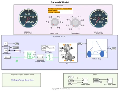
Throttle and brake input is given during runtime and the following results were observed:

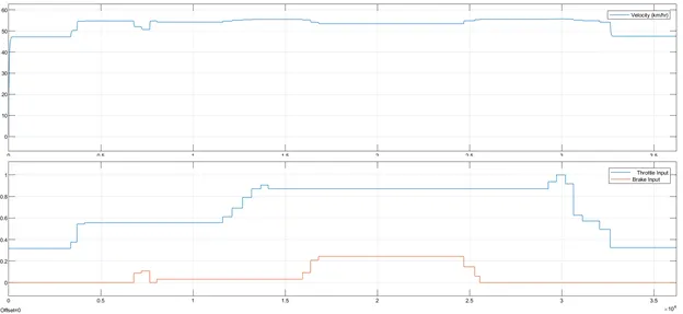
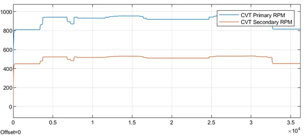
Increasing the brake input decreases the speed and increasing the throttle increases the speed and vice versa.

3. BAJA ATV closed loop model

This model uses a lookup table inside the CVT subsystem which decides the gear ratio according to the velocity fed back to the subsystem.

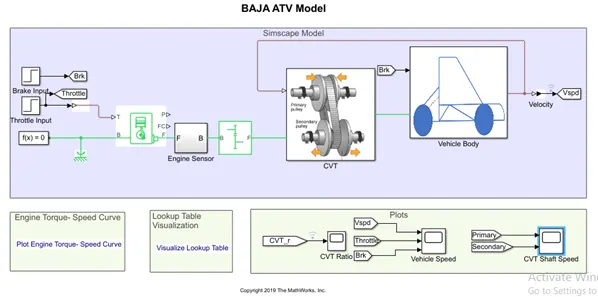
CVT Subsystem:

The results are shown below:

The explanation for the results is similar to that of the first model. But the use of lookup table improves the accuracy and smoothness of the curves.

4. BAJA ATV closed loop model and with Dashboard

This model uses a dashboard to get input during the runtime and a lookup table for getting the CVT Ratio.

Results:

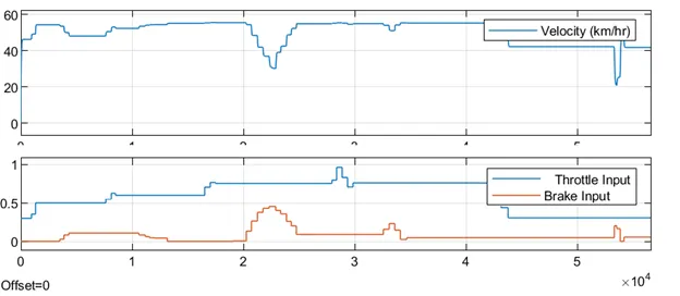
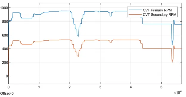
The speed varies as per the throttle and brake input. The secondary rpm follows the primary rpm linearly. Here , even if data for some values of velocity might be unavailable, the CVT ratio is still defined.

CONCLUSION:

1. As the throttle increases, the power input in the form of fuel to the engine increases and this in turn increases the rpm i.e. velocity of the shaft.
2. The output speed i.e. the secondary rpm depends on brake (inversely proportional), throttle (directly proportional) and CVT Ratio (inversely proportional) at that instant.
3. Look up tables can extrapolate and intrapolate the missing data points of the curve.
4. Dashboard elements can take instantaneous input provide instantaneous output.