Week 11- Broadband Noise modelling over Ahmed body

Aim:

1. Describe Ahmed's body and its importance.
2. Setup the domain and set up assuming the body is travelling at 110 kmph
3. Run the setup till convergence and plot for static pressure and coefficient of drag and lift to check for convergence
4. Turn on Broadband- modelling and detail the acoustic field study over Ahmed's body.

1. Introduction:

• Aerodynamics:
  • Aerodynamics is the branch of science that deals with the movement of a gaseous fluid such as air and with forces acting on the body such as a car in motion relative to the fluid.
  • It is necessary to understand the movement of air around the body in order to calculate the forces and moments acting on it.
  • For this purpose velocity, pressure and temperature are calculated for a flow field (air around a body) as a function of position and time.
  • Figure 1 shows that the movement of air over the roof of car is separated at the end of the roof; a phenomenon known as the wake. The wake is a low-pressure zone and its location is behind the car.

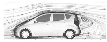
Figure 1: Flow visualisation by computer simulation

Different near-end shapes:

• Reynolds Average Navier Stokes (RANS) was used to calculate the drag coefficients.

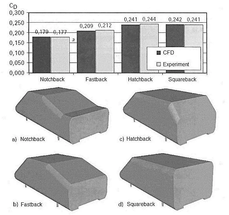
Figure 2: The four types of rear-end shapes of road vehicles with a measured and simulated drag coefficient

S. No.	Type	Application
a)	Notchback	Family car. The shape of this car design is the most streamlined shape.
b)	Hatchback	Supercar. The wake area for this car design is small.
c)	Fastback	Small family car
d)	Squareback	SUV, Vanes, and Buses. The wake area for this design is large.

Figure 3 shows the effect of the shape of the front and rear of the vehicle in Lay’s study of 1933. Obviously, the rear end shape of the vehicle has a greater influence on the drag coefficient.

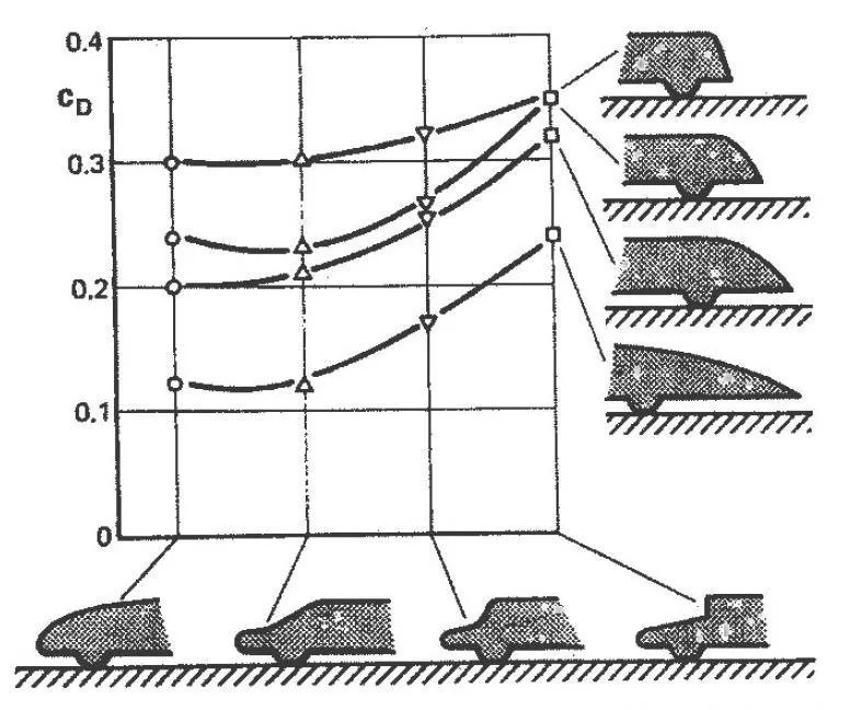
Figure 3: Summary of the test results by Lay

Conclusion:

• The shape of the rear of the car is more important than the shape of the front because of the wake.

Ahmed model:

• Automotive aerodynamic studies started by using simplified models such as the Ahmed model. Figure 4 illustrates the standard geometry of the Ahmed model and its dimensions.
• Ahmed created this geometry in 1984 and it has become a benchmark to study the main features of aerodynamic behaviour for road vehicles.
• Ahmed model is also used to study the behaviour of turbulent flow over simple car geometry.
• The Ahmed model is simple and free from all kinds of accessories as well as wheels; nevertheless, it can be used to study the aerodynamic behaviour of a road vehicle based on the main features such as the slanting surfaces.

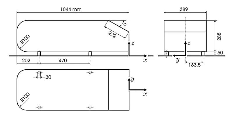
Figure 4: Standard geometry of Ahmed model

3. Effect of drag:

• All drag coefficients for road vehicles are positive. Reducing the drag coefficient implies a reduction in fuel consumption. hence all researchers and car companies aim to reduce `C_D`as much as possible.
• `C_D=(2F_D)/(rhov^2A)`

Effect of lift:

• The lift coefficient is more complex to understand because it can be positive or negative. positive lift coefficient indicates to less stability of the vehicle on the road. The negative lift coefficient implies more stability of vehicles on road but on the other hand, a high negative lift coefficient can lead to an increase the rolling resistance which increases fuel consumption.
• `C_L=(2F_L)/(rhov^2A)`

As we know, `R_e=(rhovL)/mu impliesrhov=(muR_e)/L`

`C_D=(2F_DL)/(muR_evA)=f(R_e)`

The conclusion from lift and drag:

• The best design of a road vehicle is when the `C_D`is as low as possible and `C_L` is negative but not by a high magnitude.

Ahmed body:

• Ahmed's model is simple and free from all kinds of accessories as well as wheels; nevertheless, it can be used to study the aerodynamic behaviour of a road vehicle based on the main features such as the slanting surfaces.

• 

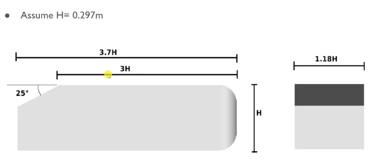
• Figure 5: Dimensions of Ahmed's body

Computational domain of the Ahmed body model:

• A rectangular cuboid is used as a computational domain as a replica of the wind tunnel. The length of the Ahmed body is L. the Ahmed model is located at a 3L distance from the inlet of the computational domain and at a 5L distance from the outlet of the computational domain. The height and width of the computational domain are 3L.
• A no-slip boundary condition is prescribed on the ground, roof and tunnel walls, while null pressure is imposed at the outlet wall.
• Half of the rectangular computational domain is used in the simulation of this work to reduce the calculation time as the whole system can be regarded as symmetric.

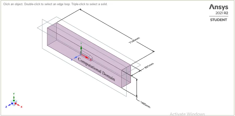
Figure 6: Isometric view of the computational domain with its dimensions

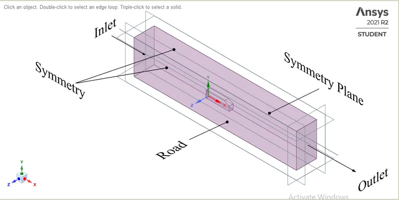
Figure 7: Parts name of Computational domain

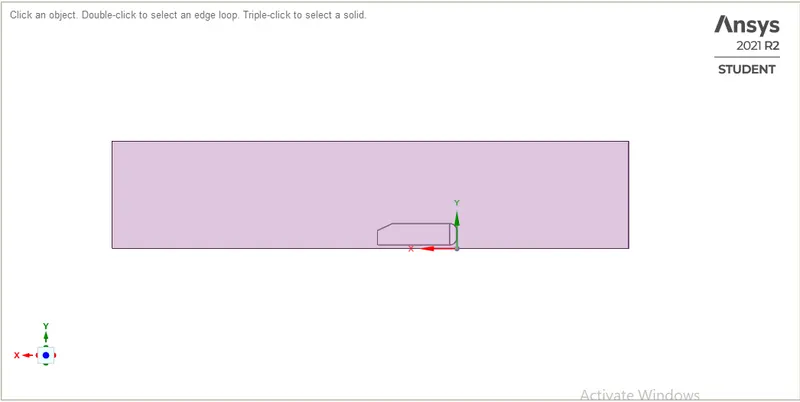
Figure 8: Backside view of Ahmed model in the computational domain.

Mesh and numerical set-up of Ahmed model:

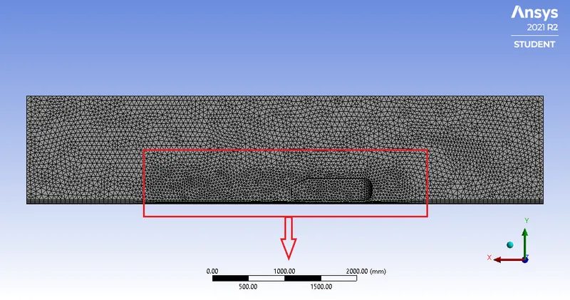
• Mesh quality is a crucial factor for obtaining accurate results in numerical study. Most researchers prefer the hexahedral mesh, especially for simple geometries, but when the quality cannot be maintained (for example orthogonal quality, skewness and aspect ratio are poor) then it is better to switch to a tetrahedral mesh. Tetrahedral mesh is a very good choice for complex geometries because the mesh cells may have any shape. This type of mesh is the most flexible type regarding geometries but it requires more mesh density than the structured grid. Increasing the mesh density means increasing of accurate results but that leads to an increase in simulation time. Therefore, the mesh density within the computational domain should be high enough to capture all flow features. It is better to improve the mesh quality before creating the prism layers around the surfaces of the geometry.
• To control the mesh growth, especially near the surfaces of the vehicle, an inner box (which is called the volumetric control region) is used. A Volumetric Control Region (VCR) with a tetrahedral mesh near the geometry is usually needed in the computational domain to improve the overall mesh quality

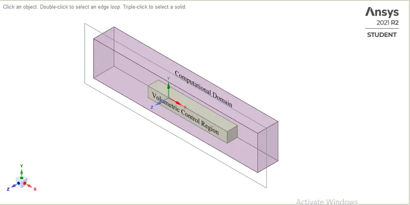
Figure 9: Created Volumetric control region near Ahmed's body to control the mesh growth

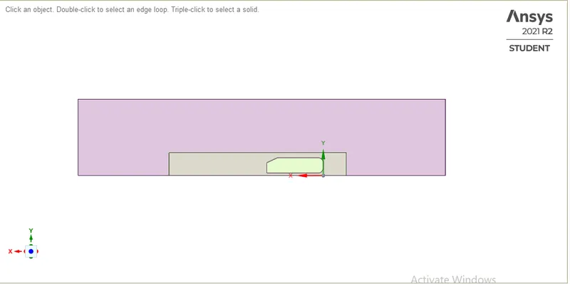
Figure 10: Backside view of Ahmed model inside control volume region in the computational domain.

Inflation layer:

• The first inflation layer near the Ahmed body and the growth rate of inflation layers is very important to know how the airflow behaves near the surface of the car.
• The concept of the y+ wall function is a dimensionless quantity representing the distance from the wall in terms of the vicious lengths.
• For the road vehicle steady-state simulation, Y+ is between 30 and 300 by using the realisable k-epsilon turbulence model.
• For more accurate results, especially near surfaces, 5 to 10 inflation (prismatic) layers are used following an analysis of the optimum number of prismatic layers.

Online Y+ Calculation:

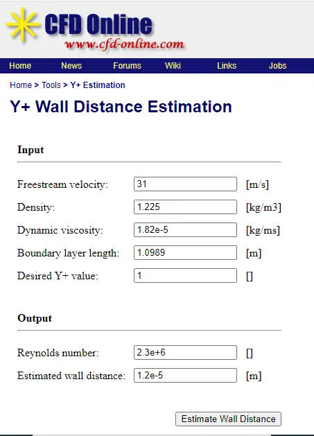
Estimated wall distance=first cell height = 1.2e-5m=0.012 mm

(OR)

Offline Y+ calculation:

step 1: Calculate Reynold Number

`R_e=(rhoU_(oo)L)/mu`

`R_e=(1.225times31times(3.7times0.297))/(1.8times10^-5)=2.318times10^6`

Step 2: Estimate the skin friction coefficient using the Schlichting skin-friction correlation:

`C_f=[2log_10(R_e)-0.65]^-2.3` for `R_e<10^9`

`C_f=[2log_10(2.38times10^6)-0.65]^-2.3=0.00323`

Step 3: Compute the wall shear stress

`tau_w=C_f1/2rhou_oo^2`

`tau_w=0.00323times1/2times1.225times31^2=1.901 N/m^2`

Step 4: Compute the shear or friction velocity

`u_star=sqrt((tau_w)/rho)`

`u_star=sqrt(1.901/1.225)=1.245 m/s`

Step 5: Compute the wall distance

`y=(y+timesmu)/(rhou_star)`

`y=(1times1.8times10^-5)/(1.225times1.245)=1.18times10^-5 m`

`y=0.011 mm`

The similarity in Reynold number and Y+ value.

S.No.	`R_e`	Y+
1.	It is a dimensionless number	It is also a dimensionless number
2.	`R_e=(rhoU_ooL)/mu`	`Y+=(rhoU_stary)/mu`

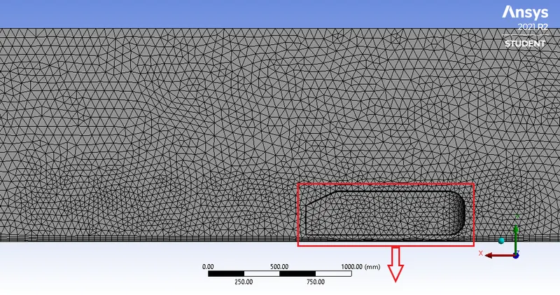
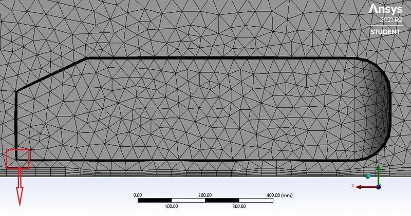
Mesh:

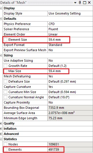
Figure: Mesh details

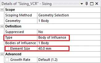
Figure: Mesh details of Volumetric control region

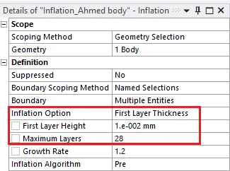
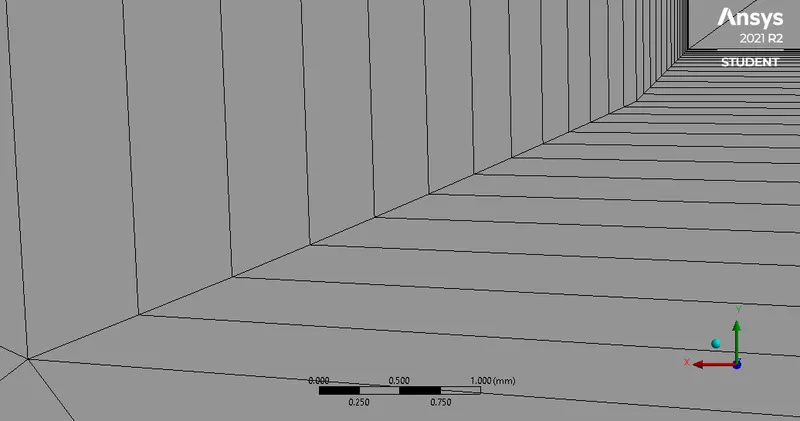
Figure: Inflation layer details on Ahmed's body

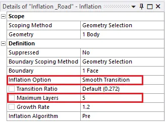
Figure: Inflation layer details on Road

1. Setup:

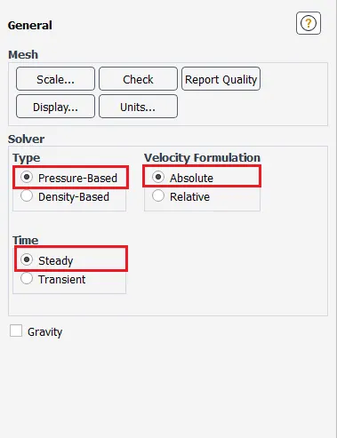
1.1Models:

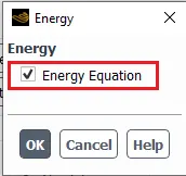
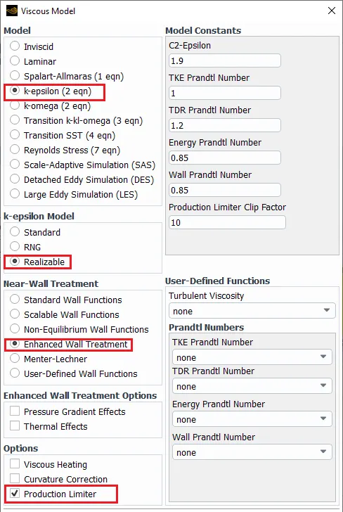
1.2 Materials:

• Fluid
  • Air
  • 

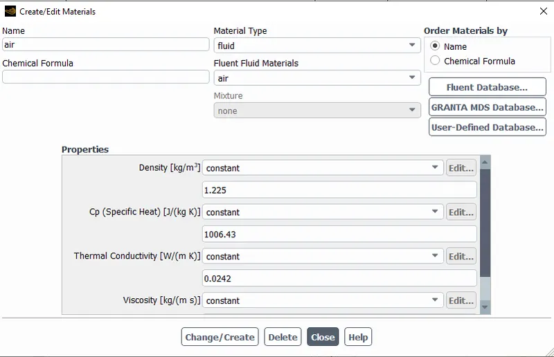
1.3 Boundary conditions:

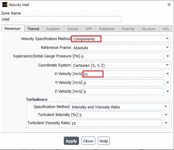
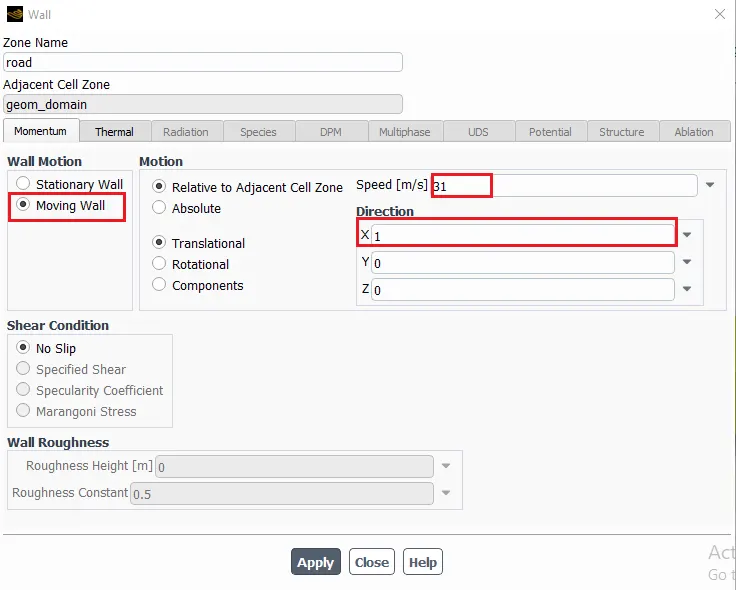
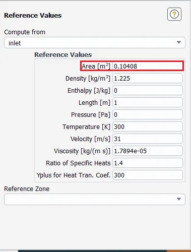
Area=Frontal area of the bluff body (from figure 5 )

Area= 1.18H*H

Area= 1.18*0.297*0.297=0.10408 square meter.

2. Solution:

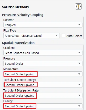
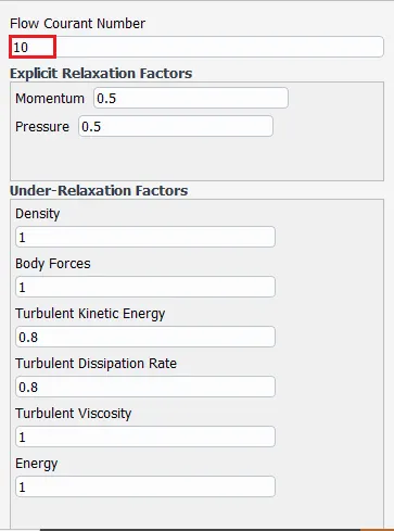
Result:

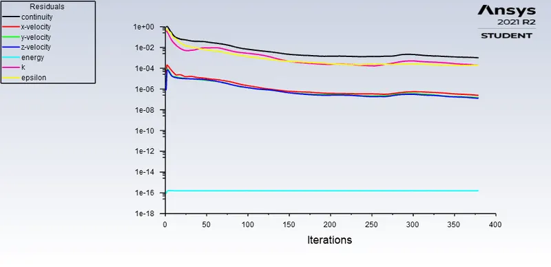
Figure: Residual plot

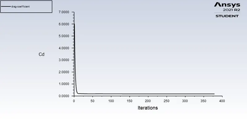
Figure: Drag coefficient plot

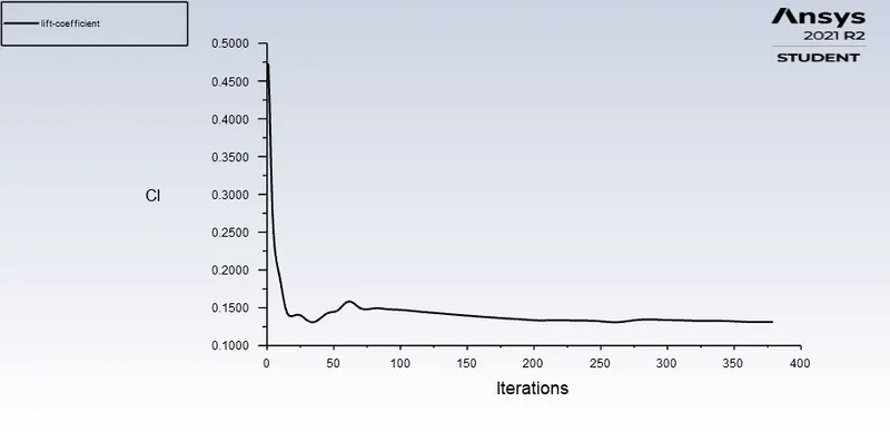
Figure: Lift coefficient plot

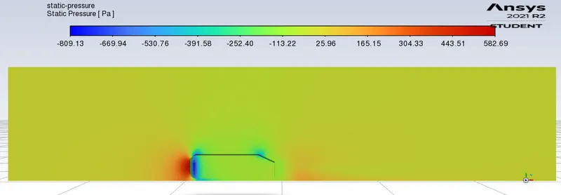
Figure: Static pressure contour

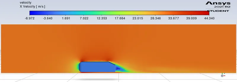
Figure: Velocity contour

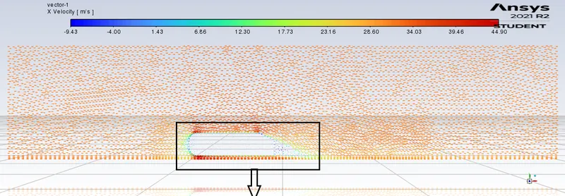
Figure: Velocity vector

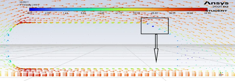
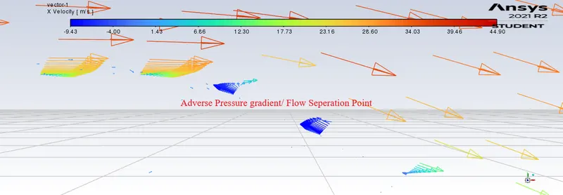
Figure: Adverse pressure gradient where the pressure value is negative.

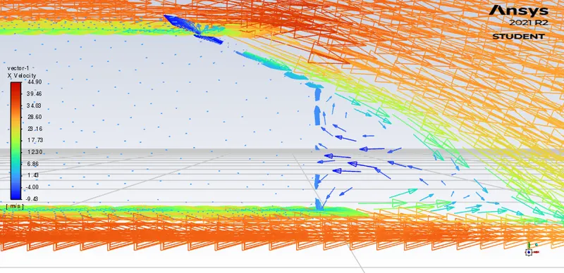
Figure: Wake region / Vortex

Predicting Aerodynamically generated noise:

Many sounds that are technologically important in industrial applications are generated by and propagated in fluid flows.

• Three approaches to computing aerodynamically generated noise.
  1. Direct approach
  2. Hybrid approach
     1. Integral method by Ffowcs Williams and Hawkings
     2. Method based on Wave equation
  3. Broadband noise source models.
     1. Proudman’s formula
     2. jet noise source model
     3. boundary layer noise source model
     4. source terms in the linearized Euler equations
     5. source terms in Lilley’s equation

Broadband noise source models:

• In many practical applications involving turbulent flows, noise does not have any distinct tones, and the sound energy is continuously distributed over a broad range of frequencies. In those situations involving broadband noise, statistical turbulence quantities readily computable from RANS equations can be utilized, in conjunction with semi-empirical correlations and Lighthill’s acoustic analogy, to shed some light on the source of broadband noise.

1. Proudman's formula:
   • acoustic power due to the unit volume of isotropic turbulence (in W/m^3) as
   • `P_A=alpharho_o(u^3/l)(u^5/a_o^5)`
   • Where `alpha` is the model constant, u is turbulence velocity, l is length scale, and `a_o` is the sound speed.
   • ANSYS Fluent can also report the acoustic power in dB, which is computed from
   • `L_p=10log(P_A/P_(ref))`
   • Where `P_(ref)` is the reference acoustic power in dB (`P_(ref)=10^-12 W/m^3` by default)

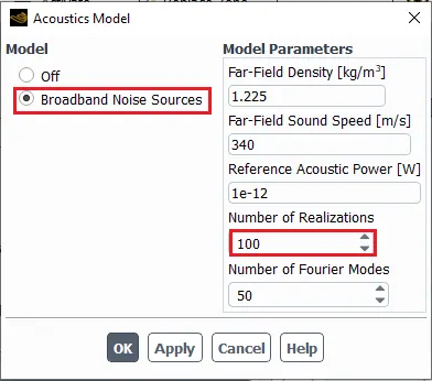
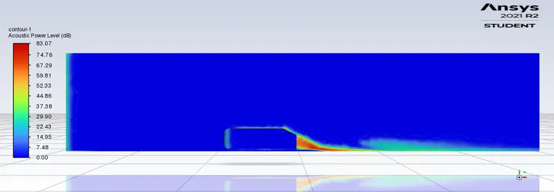
Figure: Acoustic Power Level Contour